7.1. A Small Collection of Proximity Graphs

In this section, we define a number of common proximity graphs and highlight some of their properties. This will usually be done by introducing a neighborhood that defines exactly when two nodes (i. e., points) are neighbors of each other. The following definitions and discussions build on [Jaromczyk and Toussaint 92].

7.1.1. Preliminary Definitions

Geometric graphs are graphs that are embedded in a metric space. Here, we will assume the space together with an L _p norm, 1 ‰ p ‰ ˆ . The length between two points x , y ˆˆ is defined as .

Let V be a set of points in . Edges are (unordered) pairs of points ( p, q ) ˆˆ V — V , denoted by pq . ^[1] In the following, the length of an edge is equal to the Euclidean distance between its two endpoints (any other metric could be used as well).

Proximity graphs are geometric graphs where the edges connect points that are in proximity to each other (or where at least one point is close to the other). If pq is an edge in such a proximity graph, then we say that p is a neighbor of q (and vice versa).

Exactly how proximity is defined depends on the type of neighborhood graph. It is always a geometric property, which, at least, involves the two points that are neighbors of each other (and, therefore, connected by an edge).

This property often involves spheres, so we define the sphere with center x and radius r as S ( x , r ) := { y ˆˆ d ( x, y ) = r }. Analogously, we define the (closed) ball B ( x , r ) := { y ˆˆ d ( x, y ) ‰ r }.

7.1.2. Definitions of Some Proximity Graphs

Unit disk graph. This is probably the neighborhood graph with the simplest definition. The set of edges of the unit disk graph, UDG ( V ), is defined as

i. e., two nodes are connected by an edge iff their distance is at most 1.

This definition is motivated by mobile ad-hoc networks, where each node (e. g., cell phone) can reach only other nodes within a certain radius ( assuming that all phones have the same transmission power).

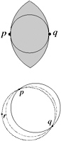
Relative neighborhood graph. We define a lune L ( p, q ) := B ( p , d ) ˆ B ( q , d ), where d = p ˆ q (see Figure 7.3).

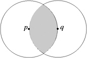
Figure 7.3: The lune is the defining neighborhood of the relative neighborhood graph.

The relative neighborhood graph (RNG) of V , RNG ( V ), is defined by the set of edges

In other words,

Or, in yet other words,

Gabriel graphs. The neighborhood here is a so-called diameter sphere , where d = p ˆ q (see Figure 7.4).

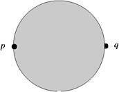
Figure 7.4: The defining neighborhood for the Gabriel graph is the diameter sphere.

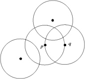
Figure 7.5: The sphere-of-influence graph is defined by spheres of influence around each point.

The Gabriel graph (GG) over V , GG ( V ), is defined by the set of edges

In other words,

-skeletons. This is a family of neighborhood graphs, parameterized by , 1 ‰ < ˆ .

For a fixed , the neighborhood is the intersection of two spheres:

where d = /2 p ˆ q . The -skeleton over V , BG ( V ), is defined by the set of edges

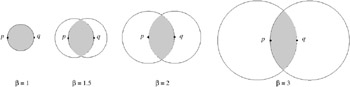
Figure 7.6: Examples of the family of lunes that define the -skeleton.

It is easy to see that RNG ( V ) = BG ₂ ( V ) and GG ( V ) = BG ₁ ( V ). Moreover, this family of proximity graphs is monotonic with respect to , i.e., ₁ > ₂ . In other words, lower values of give denser graphs.

Sphere-of-influence graph. The sphere-of-influence graph (SIG) seems to be less well-known [Michael and Quint 03, Boyer et al. 00, Jaromczyk and Toussaint 92].

While in the previous two graphs, the neighborhood is defined between pairs of points, here, the neighborhood, its sphere of influence, is defined for each point individually. More precisely, for each point p ˆˆ V , the radius r _p to its nearest neighbor is determined. Then the SIG over V , SIG ( V ), is defined by the set of edges

The SIG tends to connect points that are close to each other relative to the local point density. In contrast, the RNG and the GG tend to connect points such that the overall edge length is small (think of cities and highways: it makes sense to connect two cities directly by a highway , unless there is a third one close by that could be connected as well by a small detour ). The extreme along that line is the minimum spanning tree (see below) that has the least overall edge length.

Another difference is that the SIG, unlike the RNG or GG, can be disconnected (see Figure 7.7). This may or may not be desired, depending on the application.

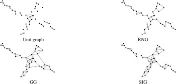
Figure 7.7: Examples of proximity graphs.

A straightforward way to reduce the likeliness or the number of gaps in the SIG is an extension, the r -SIG, r ˆˆ [Klein and Zachmann 04b]. Here, the sphere of influence is not determined by the nearest neighbor, but by the r th nearest neighbor. Obviously, the larger r , the more points that are directly connected by an edge (see Figure 7.8).

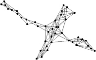
Figure 7.8: The 3-SIG over the same point cloud as in Figure 7.7.

A further extension can be applied to the r -SIG, if it is too dense or contains edges that are too long. This is pruning of edges based on a statistical outlier detection method over the lengths of edges [V. Barnett 94]. In statistics, an outlier is a single observation that is far away from the rest of the data. One definition of far away in this context is larger than Q ₃ + 1 . 5 IQR , where Q ₃ is the third quartile ( Q ₂ would be the median), and IQR is the interquartile range Q ₃ ˆ Q ₁ . Our experiments showed that best results are achieved by pruning edges with length of at least Q ₃ + IQR [Klein and Zachmann 04b]. Figure 7.9 shows the pruned 3-SIG of the example point set.

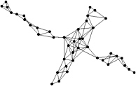
Figure 7.9: The 3-SIG with additional pruning.

Another extension could be to use ellipsoids instead of spheres [Klein and Zachmann 04b]. Then, we have the additional degree of freedom of the orientation of the ellipsoids. For instance, we could orient them along the direction of local largest variance. Depending on the application, this could have the advantage of better separating close sheets.

Other geometric graphs. There are other geometric graphs that are more or less closely related to proximity graphs, such as the minimum spanning tree and the Delaunay graph.

The minimum spanning tree (MST) spans (i.e., connects) all points by a tree (contains no cycles) of minimal length. Thus, although this tree can reveal interesting structure in the point set, there is no local proximity criterion for a pair of points.

The Delaunay graph (DG) is the dual of the Voronoi diagram (see Section 6.1.2). Alternatively, we can define the DG as follows .

Definition 7.1. (Delaunay graph.) Two points p and q are connected by an edge if they satisfy the empty circle property . The points p and q satisfy the empty circle property iff there is a circle (or, in ^d , a hypersphere) such that p and q are on its boundary and no point of V is in the interior of this circle. ^[2]

Actually, this definition is equivalent to the one given in Section 6.1.2. For the sake of uniqueness, we assume that all points are in general position , meaning that in ^d , no d + 1 points lie on a common hyperplane, and no d + 2 points lie on a common hypersphere. Figure 7.10 shows the DG and the MST for the same point set as in Figure 7.7.

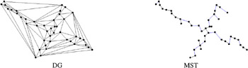
Figure 7.10: Example DG and MST for the same set of points as in Figure 7.7.

7.1.3. Inclusion Property

Here, we demonstrate the following:

Lemma 7.2. For a given set of points V,

This implies, in particular, that RNG ( V ) and GG ( V ) are connected, and that MST ( V ) ‰ RNG ( V ) ‰ GG ( V ) ‰ DG ( V ). Furthermore, in ² , the number of edges is linear in the number of points.

Proof: The proof is fairly simple. Assume for the moment that V ² .

MST ( V ) RNG ( V ) : Assume, for the sake of contradiction, that some edge pq is in the MST but not in the RNG. Then, the lune formed by p and q is not empty, i. e., there is some other point r ˆˆ L ( p, q ). But then, d ( p, r ) < d ( p, q ) and d ( q,r ) < d ( p, q ). As a consequence, the original MST is not minimal, which can be seen as follows. The original MST cannot contain both eges pr and qr ( otherwise , it would contain a cycle). If edge pr is not there, we can replace pq by pr , and have constructed a tree with smaller total edge length. Similarly, we can replace pq by qr if edge qr is not there yet.

RNG ( V ) GG ( V ) : Assume that pq is an edge in RNG ( V ). Then the lune defined by p and q is empty, and so is the diametric circle defined by p and q , since it is contained in the lune.

GG ( V ) DG ( V ) : Assume that pq is an edge in GG ( V ). Then, the diametric circle defined by p and q is empty. Thus, the pair ( p, q ) also satisfies the empty circle property as defined by Definition 7.1. Usually, the DG has more edges than the GG. This can be seen as follows. Imagine that the circle can slide to the left or right, such that its diameter increases just so that p and q always stay on its boundary (of course, it wont be a diametric any more). Because of the definition of the GG, we can slide the circle, at least a little bit, and at least to one side, without hitting another point. Now, imagine that we slide the circle until it hits a third point, r . So, we have now found two more pairs of points, ( p, r ) and ( q,r ), that satisfy the empty circle property. ^[3]

In higher dimensions, the proofs work just the same (with hyperspheres instead of circles).

7.1.4. Construction Algorithms

GG and RNG. We start with a simple algorithm for constructing the GG over a set V of points. From Lemma 7.2, we know that we can start with DG ( V ), and then remove those edges that are not neighbors according to the diameter circle property. In a brute-force algorithm, we could check this property for an edge pq of DG ( V ) by just testing each point of V to see whether it is inside the diameter circle of pq . A more efficient algorithm is to test only the neighbors of p , and those of q , against a candidate diameter circle. This is summarized in Algorithm 7.1.

Similarly, we can construct the RNG ( V ) by starting with the DG ( V ). Then we consider each edge pq of it in turn and check if there is any other point r ˆˆ V that falls inside the lune made by p and q ; i. e., if

(7.1)

Algorithm 7.1: Simple algorithm to construct the GG, starting from the Delaunay graph of a set of points.

 construct  DG  (  V  ), set  GG  :=  DG  (  V  )  for all  edges  pq     GG   do   for all  neighbors  r  of  p  or  q   do   if   r  inside diameter circle of  p  and  q   then  delete edge  pq  from  GG   end if   end for   end for

Another way to construct the GG would be by using the brute-force approach. We can consider each potential pair of points ( p, q ) (there are O ( n ² ) of them). For each of them, we check whether there is any other point r (there are O ( n )) that is inside their diametric sphere. This test essentially involves two distance computations ; i. e.,

which takes time O ( d ) in d -dimensional space. Overall, this brute-force approach would take O ( dn ³ ).

We can easily improve on this by the following observation. When checking the pair ( p, q ) to see whether they are neighbors in the GG, we must test whether any other point r is inside the diametric sphere (see Figure 7.11, left image). At the same time, we can check whether r is in the right half-space of the plane H _qp that is orthogonal to the diameter pq and goes through q . If it is, then it cannot be a Gabriel neighbor to point p (because q would be inside the diametric sphere of pr ).

Algorithm 7.2: Simple algorithm and heuristic to build the GG.

  for all   p     V   do   N  _p    V  \  p   for all   q     N  _p  do   for all   r inV   do   if  Eq. 7.1 true  then  consider next  q   else   if   r  is to the right of  H  _qp  then  remove  r  from  N  _p  end if   end if   end for   end for   end for

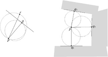
Figure 7.11: A simple heuristic leads to an O(dn ² ) algorithm to construct the GG.

So a better algorithm is the following. For each point p , we keep a list of neighbor candidates, N _p (initially, this is the whole point set). Then, as we test q _i ˆˆ N _p for being a real neighbor, we remove all r from N _p that are to the right of H _qip (see Figure 7.11, right image). This reduces the average compexity to O ( dn ² ). Algorithm 7.2 summarizes this heuristic.

The algorithm to construct the relative neighborhood graph is analogous to the one for constructing the GG.

SIG. Here, we demonstrate the following.

Lemma 7.3. The r-SIG can be determined in time O ( n ) on average for uniformly and independently point-sampled models with size n in any fixed dimension. Moreover, it consumes only linear space in the worst case.

Proof: [Dwyer 95] proposed an algorithm to determine a SIG in linear time in the average case for uniform point clouds. As r is constant, this algorithm can easily be modified so that it can also compute the r -SIG in linear time. The algorithm consists of three steps.

First, the algorithm identifies the r -nearest neighbors of each point by utilizing the spiral search proposed by [Bentley et al. 80]: the space is subdivided into O ( n ) hypercubic cells, the points are assigned to cells , and the r -nearest neighbors of each point p are found by searching the cells in increasing distance from the cell containing p . As O (1) cells are searched for each point on average and a single query can be done in O (1) [Bentley et al. 80], this first step can be done in time O ( n ).

Algorithm 7.3: Simple algorithm to compute the r-SIG in O(n) time on average.

 initialize grid with n cells  for all   p     V   do  assign  p  to its grid cell  end for   for all   p     V   do  find  r  th nearest neighbor to  p  by searching the grid cells in spiral order around  p  with increasing distance  end for   for all   p     V   do   for all  cells around  p  that intersect the sphere of influence around  p  (in spiral                  order)  do  assign  p  to cell  end for   end for   for all  cells in the grid  do   for all  pairs  p  _i  , p  _j of points assigned to the current cell  do   if  spheres of influence of  p  _i and  p  _j intersect  then  create edge  p  _i  p  _j  end if   end for   end for

Second, each point is inserted into every cell that intersects the r -nearest-neighbor sphere. On average, most spheres are small so that each point is inserted into a constant number of cells, and a constant number of points is inserted into each cell.

Finally, within each cell, all pairs of points that have been assigned to this cell are tested for intersection of their spheres of influence. Because each cell contains only a constant number of points, this can also be done in time O ( n ).

[Avis and Horton 85] have shown that the 1-SIG has at most c n edges where c is a constant. This c is always bounded by 17 . 5 [Avis and Horton 85, Edelsbrunner et al. 89]. [Guibas et al. 92a] extended this result to the r -SIG over a point cloud from ^d and showed that the number of edges is bounded by c _d r n , where the constant c _d depends only on the dimension d . That means the r -SIG consumes O ( n ) space in the worst case.

Moreover, as mentioned in [Toussaint 88], ElGindy has observed that the line-segment intersection algorithm introduced [Bentley and Ottmann 79] can be used to construct a SIG in the plane in O ( n log n ) time in the worst case. The algorithm of [Guibas et al. 92a] constructs the r -SIG in time

for any > 0 in the worst case.

^[1] Technically, one should distinguish between the combinatorial structure of the graph, given by V and the set of edges E V — V , and the geometrical realization , given by points that have an actual location in space and edges that are straight line segments connecting the points. In the following, we will not differentiate between those two.

^[2] Then, there is also a maximal empty hypersphere that has exactly d + 1 points on its boundary, two of which are p and q .

^[3] Because we always assume V to be in general position (see Definition 7.1).