6.4. Applications of the Voronoi Diagram

6.4.1. Nearest Neighbor or Post Office Problem

We consider the well-known post office problem. For a set S of sites in the sphere and an arbitrary query point q , we want to compute the point of S closest to q efficiently .

In the field of computational geometry, there is a general technique for solving such query problems. One tries to decompose the query set into classes so that every class has the same answer. Then, for a single answer, we need to determine only its class. This technique is called the locus approach .

The Voronoi diagram represents the locus approach for the post office problem. The classes correspond to the regions of the sites. For a query point q , we want to determine its class/region and return its owner.

We present some simple ideas for the region query, which work in 2D and 3D.

Decomposition of the diagram by slabs. To solve the given task, the following simple slab method can be applied. The slab method was mentioned first in [Dobkin and Lipton 76]. It subdivides the cell decomposition into slabs S _i and, in turn , every slab is subdivided by a set of segments s _i ; see Figure 6.21.

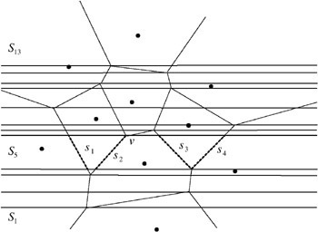
Figure 6.21: After constructing a sorted list of slabs and a sorted list of segments in every slab, a query point q can be located quickly by a binary search.

The following is the slab method sketch:

Draw a horizontal line through every vertex of the diagram and sort the lines in O ( n log n ) time; see Figure 6.21. The lines decompose the diagram into slabs ;
For every slab , sort the set of crossing edges of the Voronoi diagram. We must trace the DCEL of the Voronoi diagram and will find a sorted set of crossing segments in linear time.

Algorithm 6.6: The construction of a slab search structure for the region query returns a 2D arrayS. For each vertical line, the array contains a sorted array of crossing segments.

SlabStructureConstr( T ) ( T represents the DCEL of the Voronoi diagram)

  V  :=  T.  GetVertices  L  :=  V.  sortByY  S  := new array(  L   ,  2)  i  := 0  while   L  =     do   S  [  i  ][1] :=  L.  First  L.  DeleteFirst  E  _L :=  T.  TraceLeft(  S  [  i  ][1])  E  _R :=  T.  TraceRight(  S  [  i  ][1])        EdgeArray := Concat(  E  _R  , E  _L )  S  [  i  ][2] := EdgeArray  i  :=  i  + 1  end while   return   S

The corresponding algorithm must return a data structure that supports a binary search. For example, we can insert the slabs into a binary tree. In turn, every tree node represents the segment subdivision of a slab by a binary tree representing segments.

Alternatively, we use a sorted array of vertical line segments, where every line entrance stems from a vertex v . The corresponding slab lies below v with respect to the y order of the lines. For example, in Figure 6.21, the fifth vertex from below, v , represents the slab S ₅ . For the highest slab, we can introduce an artificial vertex at + ˆ . Additionally, for every line segment in the sorted array, we store a sorted array of the segments crossing the corresponding slab; see Figure 6.21 and compare to Algorithm 6.6. The full structure can be represented in an ( n — n )- dimensional 2D array S , where S [ i ][1] denotes the Voronoi vertex and S [ i ][2] contains an array of sorted segments. For example, in Figure 6.21 the slab S ₅ is given by S [5][] with S [5][1] = v and S [5][2] = [ s ₁ , s ₂ , s ₃ , s ₄ ].

Algorithm 6.7: The region query can be answered efficiently using a slab decomposition and a binary search.

SlabQuery( S, V, q ) ( S represents the 2D region query array computed by Algorithm 6.6, V represents the DCEL of the corresponding Voronoi diagram, and q is a query point)

  j  :=  S.  BinSearchAbove(  q  _y )  e  :=  S  BinSearchLeft(  q  _x )  p  :=  V  ReportRightRegion(  e  )  return   p

Tracing through the DCEL as indicated by TraceLeft or TraceRight in Algorithm 6.6, compute the array of segments of the current slab. The trace can be done in linear time as follows . In the planar DCEL, we sucessively check the edges of the corresponding face of the current vertex and test for intersections. Thus, we will find the first intersection. Then we go on recursively with the next face using the corresponding pointers in the DCEL; see Section 9.1.1. See also Algorithm 6.8. Altogether, we need O ( n ) time for computing a sorted array of line segments for a single slab, and O ( n ² ) time for computing all slabs.

We can speed up the construction by the following idea. From one slab to the next slab, only a single vertex and its outgoing edges has to be considered , because the sorted array of segments can only change locally. If the sorted array of segments S [ i ][2] for a slab i is constructed , the next sorted array for vertex S [ i + 1][1] is computed from S [ i ][2] and the outgoing edges at S [ i + 1][1]. Thus, the next array of segments is constructed in time proportional to the degree of the corresponding node, which equals 3 in the Voronoi diagram.

Altogether, the incremental construction of the slabs takes O ( n ) time but O ( n ² ) space is required. In the corresponding algorithm, the operations T. TraceLeft( S [ i ][1]) and TraceRight( S [ i ][2]) will use the information of S [ i ˆ 1][2]. Only the first slab has to be constructed from scratch. Note that presorting of the vertices and the construction of the Voronoi diagram result in O ( n log n ) construction time altogether.

A query is done efficiently as follows. For a query point q , we locate its slab in O (log n ) time and then its region in O (log n ) time, both by binary search.

For reporting the region of a query, it suffices to find the appropriate line or edge below p or to the left of q , rather than the slab or the region itself. This is indicated in Algorithm 6.6 by BinSearchAbove, BinSearchLeft, and ReportRightRegion. For example, S. BinSearchAbove( q _y ) returns index j if q lies between the slabs S [ j ][] and S [ j + 1][], assuming that the slabs are ordered by increasing y -coordinates of the vertices.

Theorem 6.8. Given a set S of n point sites in the plane, one can, within O ( n log n ) time and O ( n ² ) storage, construct a data structure that supports nearest neighbor queries. For an arbitrary query point q, its nearest neighbor in S can be found in time O (log n ) .

It was shown already in [Cole 86] that we do not need to consider a unique data structure for every slab, because only one segment changes from one slab to the other. This key idea was used in [Sarnak and Tarjan 86] for the persistent search tree model. In this model, we start with an empty search tree and insert the crossing segments sucessively. There is a linear size tree data structure that stores the changes over time and gives access to every structure in constant time. See also [Edelsbrunner 87].

The presented ideas can be extended to 3D. We can analogously subdivide the 3D diagram into slabs by horizontal planes at the vertices. Unfortunately, the given slabs will still contain convex 3D objects; see Figure 6.22 for a simple example of a slab. Therefore, we need a data structure for handling queries in 3D slab subdivisions, which is the subject of the next section. The methods of the next section can be applied also to the 2D Voronoi diagram and also to the full 3D Voronoi diagram.

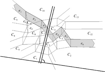
Figure 6.22: The separating surfaces for a 3D slab subdivision of convex cells . The separator ƒ ₁₀ separates the cells C ₁ , C ₂ , , C ₁₀ from C ₁₁ , C ₁₂ , , C ₁₄ .

Separating surfaces for 2D and 3D point location in a convex cell decomposition. Let us assume that we have a cell decomposition with convex cells as shown in Figure 6.22. The cells can be ordered as follows. We move a hyperplane perpendicular to the x -axis and parallel to the y -axis along the x -axis. Let H _x denote the corresponding intersection with the given 3D slab at position x ; see Figure 6.22. H _x suggests a partial order of the neighboring cells as follows.

If C and D share a boundary face and C lies below D with respect to the corresponding hyperplanes H _x , then let C ‰ D . The relation ‰ is acyclic because the cells are convex. Then we can easily extend the partial order to a total order of all cells. This means that we enumerate the cells by C ₁ , C ₂ , , C _k , so that C _i ‰ C _j implies i < j .

For every i , there is a sequence of surfaces that splits C ₁ , C ₂ , , C _i from C _i ₊₁ , C _i ₊₂ , , C _k ; see Figure 6.22 for an example for i = 10. Let ƒ _i denote this separator ; see also [Tamassia and Vitter 96] and [Edelsbrunner et al. 84]. The separators ƒ _i and ƒ _i ₊ ₁ differ in surfaces belonging to C _i . We can build a binary tree for the separators due to their numeration; see Figure 6.24.

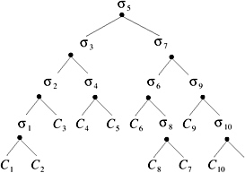
Figure 6.24: The binary separator tree for the cell decomposition of Figure 6.25. Every leaf represents a cell.

The intention is that by a binary search we want to find the separators ƒ _i and ƒ _i ₊ ₁ , so that the query point lies between them in a unique cell. In turn, for every separator, we should be able to decide whether the query point lies below or above the separator. This is very similar to the slab method. Fortunately, we can use the properties of the Voronoi diagram. The Voronoi cells were constructed by the intersections of hyperplanes. Therefore, they are convex, and every separator is an x -monotone chain by construction. This means that we can answer the above/below separator query by a binary search also. For the x -monotone separator, we can build a binary tree of its edges; see Figure 6.23 for the separator ƒ ₁₀ in Figure 6.22.

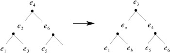
Figure 6.23: The separator ƒ ₁₀ of Figure 6.22 is a binary tree of its edges. From ƒ ₁₀ to ƒ ₉ , local updates are made.

Altogether, we have to construct a binary tree of separators, and for every separator, construct a binary tree of its surfaces. The binary tree of separators contains a single cell at every leaf of the tree. The path from the root to the leaf of the tree shows how this cell is enclosed by separators. If the order of the separators is given, we can build up the binary tree easily. For example, Figure 6.24 shows the binary separator tree for the cell decomposition of Figure 6.25.

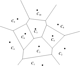
Figure 6.25: The y order of the Voronoi sites gives the total order of the cell decomposition in 2D and 3D.

Finally, we consider the construction of the separators. The presented idea works also for the Voronoi diagram in 2D and is more elegant as the simple slab subdivision. For convenience, we illustrate the construction in 2D; that is, surfaces are replaced with edges. Fortunately, a total order of the cells is obviously given by the y order of the sites; see Figure 6.25. This is also true in 3D. We assume that no two points have the same y -coordinate. Otherwise, we can apply the methods presented in Section 9.5.

With the help of the Voronoi diagram, the separators are constructed incrementally. Let a total order C ₁ , C ₂ , , C _k , so that C _i ‰ C _j implies i < j be given by increasing y -coordinates of the sites. For every C _i , the corresponding site is known.

The following is the separator construction sketch:

The first ƒ _k separator for C _k and C ₁ , C ₂ , , C _k _ˆ1 is given by the boundary of C _k . The edges are given in x -monotone order. Build a binary tree of the edges and keep a reference to the DCEL of VD( S ) for every edge;
Assume that the separator ƒ _i _ˆ ₁ is already constructed for C _i _ˆ ₁ , C _i , , C _k and C ₁ , C ₂ , , C _i _ˆ2 , and a binary tree of the edges is given.
- For C _i , delete the subchain of edges of which are already in the tree of ƒ _i _ˆ1 ;
- Insert the subchain of edges of which were not in the tree of ƒ _i _ˆ1 . The order of the whole chain and the balance of the tree must be maintained .

For example, the incremental reconstruction step in 3D from separator ƒ ₁₀ to ƒ ₉ in Figure 6.22 deletes the edge e ₂ and inserts the chain e _a and e _b ; see Figure 6.23 for the corresponding trees.

The running time of the construction of the separators depends on the complexity of the cell decomposition. If the cell decomposition has O ( m ) faces, then the trees are constructed in O ( m log m ) time due to the insertion and the deletion of O ( m ) edges. The number of edges in all separators is obviously quadratic in m . A point location query for a point p is answered by a binary search in O (log m ) time as follows.

The following is the point location query sketch:

Consider the root node v of a binary tree of separators and the corresponding separator ƒ ;
If v is a leaf, report the corresponding cell;
Otherwise check whether p lies below or above ƒ as follows:
- Consider the root w of the binary tree of edges of ƒ and the corresponding edge e ;
- Check whether p lies in the corridor spanned by two vertical lines passing through the left and right endpoints of e . If this is true, check whether p lies above or below e and return this value;
- Otherwise, if p is not in the corridor of the left and right endpoints of e , branch to the child of w of the segment tree that lies on the same side as p with respect to the corridor at e . Repeat the process with this child and its associated edge (the new w and e );

If p lies below ƒ , branch to the child of v that contains the separator below ƒ . Otherwise, branch to the child of v that contains the separator above ƒ . Repeat the process with this child (the new v ).

The presented approach works in the same way in 3D and also on the full 3D Voronoi diagram also; that is, we can neglect the slab structure for 3D. In the point location query, the edges are replaced by surfaces and the corridor check is done for an area separated by three halfspaces. Altogether, the following result holds.

Theorem 6.9. For a Voronoi diagram cell decomposition in 3D with O ( m ) faces, there is a data point location structure based on separators that can be built up in O ( m log m ) time and O ( m ² ) space. A point location query can be answered in O (log m ) time.

Finally, we present a very simple method for the nearest-neighbor query.

Algorithm 6.8: Answering a region query by tracing a line through the DCEL.

TraceLine( V, p _f , f, q ) ( V represents the DCEL of a Voronoi diagram, q is a query point, and p _f is an arbitrary point on a face f of V .)

  P  :=  V.  polyhedron(  p  _f  , q  ) (  p  _f  , f  ):=  V.  TraceExit(  P, p  _f  , q  )  if   p  _f = Nil  then   return  ReportSite  (   P  )  else  TraceLine(  V, p  _f  , f, q  )  end if

Tracing a line in the diagram. Another very simple method for the locus approach and the nearest neighbor problem is tracing a line from a specified vertex to the query point. This simple method works in arbitrary dimension and needs no preprocessing. Let the DCEL V of the Voronoi diagram and a query point q be given.

The following is the line tracing sketch:

Choose an arbitrary point p _f on a face f of the Voronoi diagram V . Consider the line l passing from p _f to q . The line passes a convex polyhedron P first;
Move around P using the DCEL until the exit point p _f of l for P on a face f of P is found;
If there is no such exit point, then report the site of P ;
Otherwise, go on with the line passing from p _f to q .

It remains to describe the operation TraceExit in Algorithm 6.8. We simply trace the boundary of a polyhedron P of V that is crossed by the ray from p _f to q first. The face f serves as the starting face. We are searching for the exit edge or face and its corresponding intersection point. In the planar DCEL, we successively check the edges of the corresponding polyhedron and test for intersection. In 3D, we also make use of the DCEL, and successively check all faces and test for intersection with the trace line.

The running time of the simple trace technique depends on the complexity of the Voronoi diagram and the chosen starting point. As noted earlier, in practical situations, the complexity of a Voronoi diagram in 3D often lies within O ( n ) for n sites. On the other hand, the expected number of steps in the tracing algorithm is given by O (log n ) if the DCEL has linear size; see [Dwyer 91], [Devroye et al. 98] and [Devroye et al. 04]. In the worst case, the presented algorithm needs O ( n ² ) time. The trace method does not need a search query data structure.

Theorem 6.10. Tracing a line through the Voronoi diagram of complexity O ( m ) has time complexity O ( m ) in the worst case, but expected time is O (log m ) .

6.4.2. Other applications of the Voronoi Diagram in 2D and 3D.

With the help of the Voronoi diagram, we can answer nearest neighbor queries between the sites efficiently. The nearest neighbors from S for a point p _i ˆˆ S lie inside a neighbor region of p _i in VD( S ). This is easy to see by the following general argument, which holds in 2D and 3D.

Let us separate S into two sets S ₁ and S ₂ . The nearest neigbors of S ₁ and S ₂ ; that is, two points p ₁ ˆˆ S ₁ and p ₂ ˆˆ S ₂ , where

share a surface in the Voronoi diagram of S and, in turn, an edge in the Delaunay triangulation. This is easy to see by the following argument. If the line segment between p ₁ and p ₂ contains a point c that belongs to a cell p ‰ p ₁ , p ₂ , then we have d ( p, c ) < d ( p ₁ , c ) , d ( p ₂ , c ). Let p ˆˆ S ₁ . By the triangle inequality, we have

which gives a contradiction to the definition of p ₁ and p ₂ .

Now, we can apply this argument for S ₁ = { p _i } and S ₂ = S \ S ₁ .

Theorem 6.11. Let S be a set of points in 3D . For the nearest neighbor p _j ˆˆ S of a point p _i ˆˆ S, there is an edge p _i p _j in the Delaunay triangulation of S. All nearest neighbors can be found in time proportional to the complexity of the Voronoi diagram.

Beyond nearest neighbor queries, there are many different geometrical applications of the Voronoi diagram and its dual. Here, we simply list a few of them, together with some performance results, provided that the diagram is given.

The Delaunay triangulation contains the minimum spanning tree . By definition, the minimum spanning tree is the smallest graph (with respect to overall edge length) that connects all sites. The algorithm of Kruskal [Kruskal, Jr. 56] computes a minimum spanning tree of an arbitrary graph G = ( V, E ) in time O ( E log E ). Therefore, the minimum spanning tree of a set of points can be computed applying Kruskals algorithm on the sparse Voronoi diagram.

Theorem 6.12. The minimum spanning tree of a set of points in 3D is part of the Delaunay triangulation.

Proof: We apply a divide-and-conquer argument. If the minimum spanning tree of S is given, we can split the tree at every edge into two disjoint subsets of sites S ₁ and S ₂ . As already shown, the edge connecting S ₁ and S ₂ has to be a Delaunay edge.

The minimum spanning tree gives us a simple heuristic for the traveling salesman problem, TSP for short. The traveling salesman visits all sites and returns to its start point. We are interested in computing the shortest tour (with respect to edge length) that solves this problem. It was shown that the problem of computing the optimal TSP tour is NP-hard. If we follow the edges of the minimum spanning tree in a depth-first manner and return to the start, we have visited every edge exactly twice. The length of the minimum spanning tree is always smaller than a TSP tour. Thus, we can compute a TSP approximation in O ( E log E ) time, where E denotes the set of edges in the Delaunay triangulation.

Theorem 6.13. Following the minimum spanning tree of a set of sites in 3D in a depth-first manner gives a 2-approximation of the optimal TSP tour of the sites.

The Voronoi diagram is helpful also for the subject of localization; see also [Hamacher 95]. Let us assume that the sites in 3D represent sources of danger, such as fire or earthquake. Then we would like to find a location inside a given convex area A so that we have maximum security. In terms of the geometry, we are searching for the biggest empty ball with respect to the sites inside A . It can be shown that the center of this ball lies on the vertices of Voronoi diagram of the set of sites or on the boundary of the considered area A .

The geometric argument is as follows. For a possible center c , we enlarge the ball by moving c until a site of S is met. If this is only a single site, we can further enlarge the ball until a second site is met. Now we are on the surface of a Voronoi region. We move along this bisector and can enlarge the ball until three sites lie on the boundary of the ball. Thus, we are located on a Voronoi edge. Now, we can still enlarge the ball, moving along the edge until finally a fourth site is met.

Within this enlargment process, we might touch the boundary of the area A at some stage. In this case, we have to find an optimal location on A . Either this location is given by an intersection with a surface or an edge of VD( S ), or c is somewhere on A if A is met in the first stage of the enlargement . Since A is convex, we will move the center toward a vertex of A in order to enlarge the ball. Altogether, the following holds.

Theorem 6.14. The biggest empty ball of a set of sites S in 3D in a given convex area A has its center c either on a Voronoi vertex of VD S or on the boundary of A. On the boundary of A, c is either an intersection of A with an edge or a surface of the diagram, or c is a vertex of A.

Additionally, for localization planning, the farthest color Voronoi diagram has some nice applications. Assume that we have subsets of sites P ₁ , P ₂ , , P _k such that P _i represents the same source; for example, P _i might represent the location of all supermarkets or all hospitals . Now, we would like to choose a location such that one instance of every source set is nearby. Geometrically speaking, we are searching for the smallest ball that contains at least one instance of every set P _i for i = 1 , , k . Let us assume that every P _i has its own color. Obviously, the optimal ball has four sites of different colors on its boundary and no other site with the same color inside the ball. Otherwise, we could shrink the ball. This means that for the center of this ball, the four sites represents the four farthest colors among all the colors. Thus, the center is a Voronoi vertex in the 3D farthest color Voronoi diagram. Altogether, we systematically check all four-colored Voronoi vertices in the given diagram.

Theorem 6.15. Let P ₁ , P ₂ , , P _k denote k point sets in 3D such that each set has its own color. The smallest ball that contains at least one instance of every set P _i for i = 1 , , k has its center on a four-colored Voronoi vertex of the farthest color Voronoi diagram.

There are many other applications, such as motion planning or clustering; see the monographs mentioned at the beginning of this section. For example, using Voronoi diagrams for clustering of objects is shown in [Dehne and Noltemeier 85].

The complexity and the running time of the corresponding algorithms depend on the complexity of the Voronoi diagram. As we have already mentioned, the complexity of the diagrams in 3D is linear in many practical situations also. Thus, many of the presented problems can be solved in 3D with almost the same time bound as in the 2D case.