2.4. Kd-Trees

In general, a windowing query considers a set of objects and a multi-dimensional window, such as a box. All objects that intersect with the window should be reported . Thus, one can easily decide which objects are located within a certain area, one of the classic problems arising in computer graphics.

The kd-tree is a natural generalization of the one-dimensional search tree considered in the previous section. It can be viewed also as a generalization of quadtrees. With the help of a kd-tree, one can efficiently answer (point/ axis-parallel box) windowing queries as follows :

Input: a set of points S in ;
Query: an axis-parallel d -dimensional box B ;
Output: all points p ˆˆ S with p ˆˆ B .

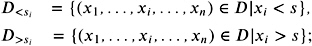
Let D be a set of n points in . For convenience, we assume that for a while k = 2, and that all x - and y -coordinates are different. If this is not the case, we will have a so-called degenerate situation, and we can apply the techniques presented in Section 9.5. Let us further assume that we have decided to split D along the x -axis, and that we have determined the split value s of the x -coordinates. Then we split D by the split line x = s into subsets

We repeat the process recursively with the constructed subsets. For every split operation, we have to determine the split axis and the split value. The simplest strategy is to choose the axes in a cyclic manner (i.e., x -, y -, z -axis, etc.)this is called a cyclic kd-tree. More precisely, a kd-tree for dimension d is constructed as follows.

The following is the inductive construction of a kd-tree sketch:

Input: given a set of points D in dimension d and the split coordinate x _i ;
If D is empty, then return an empty node v ;

Otherwise, allocate a node v for the root of the kd-tree with two children v. LeftChild and v. RightChild. Choose a split value s _i with respect to the chosen coordinate x _i . Split the set D into subsets

Algorithm 2.9: Recursive construction of a kd-tree.

KdTreeConstr( D, i ) ( D is a set of points in , i ˆˆ {1 , , d })

  if   D  =     then   v  := Nil  else   v  := new node  if   D  = 1  then   v.Element  :=  D.Element   v.  LeftChild := Nil  v.  RightChild := Nil  else   s  :=  D.  SplitValue(  i  )  v.  Split :=  s v.  Dim :=  i   D  _<s :=  D.  Left(  i, s  )  D  _>s :=  D.  Right(  i, s  )  j  := (  i  mod  d  ) + 1  v.  LeftChild := KdTreeConstr(  D  _<s  , j  )  v.  RightChild := KdTreeConstr(  D  _>s  , j  )  end if   end if   return   v

Recursively, build the kd-trees v. LeftChild and v. RightChild for the set D _<s and D _>s with respect to the next coordinate x _j , j = ( i mod d ) + 1, respectively. Finally, return the node v .

The tree will be built up by KdTreeConstr( D, 1). Thus, we simply obtain a binary tree. The balance of the tree depends on the choice of the split value in procedure SplitValue. In case of d = 2, we obtain a 2D kd-tree ^[2] of the point set D ; see Figure 2.6. Each internal node of the tree corresponds to a split line. For every node v of the kd-tree, we define the rectangle R ( v ), the region of v , which is the intersection of half-planes corresponding to the path from the root to v . For the root r , R ( r ) is the plane itself; the children of r , say and , correspond to two half-planes R ( ) and R ( ), and so on. The set of rectangles { R ( l ) l is a leaf} gives a non-overlapping partition of the plane into rectangles. Every R ( l ) has exactly one point of D inside. We do not have to store the rectangles explicitly; they are given by the path from the root to the corresponding node; see Figure 2.6.

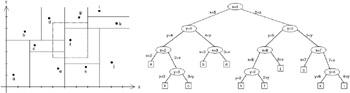
Figure 2.6: A 2D kd-tree and a rectangular range query. Each node corresponds to a split line. Additionally, each node represents a unique rectangular range R(v) according to the path from the root to the node.

For simplicity, we again consider the 2D case. The kd-tree in 2D efficiently supports range queries of axis-parallel rectangles. If Q is an axis-parallel rectangle, the set of sites v ˆˆ D with v ˆˆ Q can be computed as follows. We have to compute all nodes v with:

If the condition holds for node v , it will hold also for the predecessor u of v in the kd-tree since R ( v ) R ( u ). Thus, we can start searching from the root to the leaves . Finally, if we reach a leaf of the tree with the given property, we still have to check whether the data point of the leaf is inside Q .

For general dimension d , every node v implicitly represents an orthogonal box in dimension d . Analogously, the box is given by the path from the root to v . For the query operation, we store the current orthogonal box explicitly during the query process. We obtain the following query procedure.

The following is the d -dimensional axis-parallel query sketch:

Input: the root r of a kd-tree in dimension d and a d -dimensional orthogonal range R . The d -dimensional orthogonal box Q ( v ) defines the range associated with node v . In the beginning, Q ( r ) represents the full d -dimensional space for the root r ;
Let v be the current node;
If v is a leaf, then check whether the element v. Element stored in v lies in R , and if so, report the element. Stop the procedure;
Otherwise, the given Q ( v ) is split into the regions Q ( v. LeftChild) and Q ( v. RightChild) for the left and the right child of v by using the split line v. Split;

If Q ( v. LeftChild) or Q ( v. RightChild), respectively, is fully contained in R , then report all points in v. LeftChild or v. RightChild, respectively;

Algorithm 2.10: The query procedure of the d-dimensional kd-tree.

KdTreeQuery( v, Q, R ) ( v is the node of a kd-tree, Q is its the associated d -dimensional range, and R is a d -dimensional orthogonal query range)

  if   v  is a leaf and  v.  Element    R   then   return   v.  Element  else   v  _l := LeftChild(  v  )  v  _r := RightChild(  v  )  Q  _l :=  Q.  LeftPart(  v.  Split)  Q  _r :=  Q.  RightPart(  v.  Split)  if   Q  _l    R   then  (  v.  LeftChild)  .  Report  else if   Q  _l    R        then  KdTreeQuery(  v.  LeftChild  ,Q  _l  ,R  )  end if   if   Q  _r    R   then  (  v.  RightChild)  .  Report  else if   Q  _r    R  =     then  KdTreeQuery(  v.  RightChild  , Q  _r  , R  )  end if   end if

If Q ( v. LeftChild) or Q ( v. RightChild), respectively, intersect with R , then rerun the procedure with v. LeftChild and Q ( v. LeftChild) or v. RightChild and Q ( v. RightChild), respectively.

For convenience, we discuss time and space complexity for the 2D case. It can be shown that in 2D, the number of nodes that fulfill R ( v ) ˆ Q ‰ ˜ is restricted to , where h denotes the depth of the tree and k denotes the number of points in Q , i.e., the size of the answer; see [Klein 05] or [de Berg et al. 00]. Altogether, the efficiency of the kd-tree with respect to range queries depends on the depth of the tree. A balanced kd-tree can be easily constructed. We sort the points with respect to the x - and y -coordinates. With this order, we recursively split the set into subsets of equal size in time O (log n ). The construction runs in time O ( n log n ), and the tree has depth O (log n ). Altogether, the following theorem can be proven.

Theorem 2.9. A balanced kd-tree for n points in the plane can be constructed in O ( n log n ) and needs O ( n ) space. A range query with an axis-parallel rectangle can be answered in time O ( + a ) , where a denotes the size of the answer.

As mentioned earlier, the 2D kd-tree can be easily generalized to arbitrary dimension d , splitting the points successively with respect to the given axes in a balanced way. Fortunately, the depth of the balanced tree still is bounded by O (log n ), and the tree can be built up in time O ( n log n ) and space O ( n ) for fixed dimension d . Therefore, the kd-tree is optimal in space. A rectangular range query can be answered in time .

Theorem 2.10. A balanced d-dimensional kd-tree for n points in can be constructed in O ( n log n ) and needs O ( n ) space. A range query with an axis-parallel box in can be answered in time , where k denotes the size of the answer.

The main advantage of the d -dimensional kd-tree lies in its small size. In the following section, we will see that rectangular range queries can be answered more efficiently with the help of range trees. A WeakDelete operation in the kd-tree can be done in O (log n ). We simply traverse the tree up to the corresponding node and mark the node as deleted.

Lemma 2.11. A WeakDelete operation for a balanced d-dimensional kd-tree for n points in can be performed in O (log n ) time.

^[2] According to [de Berg et al. 00], the term k-d tree was meant as a template to be specialized like 2-d tree, 3-d tree, etc. Today, it is customary to specialize it like 2D kd-tree, etc.