10.3 Image segmentation

10.3 Image segmentation

If VOPs are not available, then video frames need to be segmented into objects and a VOP derived for each one. In general, segmentation consists of extracting image regions of similar properties such as brightness, colour or texture. These regions are then used as masks to extract the objects of interest from the image [4]. However, video segmentation is by no means a trivial task and requires the use of a combination of techniques that were developed for image processing, machine vision and video coding. Segmentation can be performed either automatically or semiautomatically.

10.3.1 Semiautomatic segmentation

In semiautomatic video segmentation, the first frame is segmented by manually tracing a contour around the object of interest. This contour is then tracked through the video sequence by dynamically adapting it to the object's movements. The use of this deformable contour for extracting regions of interest was first introduced by Kass et al. [5], and it is commonly known as active contour or active snakes.

In the active snakes method, the contour defined in the first frame is modelled as a polynomial of an arbitrary degree, the most common being a cubic polynomial. The coefficients of the polynomial are adapted to fit the object boundary by minimising a set of constraints. This process is often referred to as the minimisation of the contour energy. The contour stretches or shrinks dynamically while trying to seek a minimal energy state that best fits the boundary of the object. The total energy of a snake is defined as the weighted sum of its internal and external energy given by:

(10.1) 

In this equation, the constants a and β give the relative weightings of the internal and the external energy. The internal energy (E_internal) of the snake constrains the shape of the contour and the amount it is allowed to grow or shrink. External energy (E_external) can be defined from the image property, such as the local image gradient. By suitable use of the gradient-based external constraint, the snake can be made to wrap itself around the object boundary. Once the boundary of the object is located in the first frame, the shape and positions of the contours can be adapted automatically in the subsequent frames by repeated applications of the energy minimisation process.

10.3.2 Automatic segmentation

Automatic video segmentation aims to minimise user intervention during the segmentation process and is a significantly harder problem than semiautomatic segmentation. Foreground objects or regions of interest in the sequence have to be determined automatically with minimal input from the user. To achieve this, spatial segmentation is first performed on the first frame of the sequence by partitioning it into regions of homogeneous colour or grey level. Following this, motion estimation is used to identify moving regions in the image and to classify them as foreground objects.

Motion information is estimated for each of the homogenous regions using a future reference frame. Regions that are nonstationary are classified as belonging to the foreground object and are merged to form a single object mask. This works well in simple sequences that contain a single object with coherent motion. For more complex scenes with multiple objects of motion disparity, a number of object masks have to be generated. Once the contours of the foreground objects have been identified, they can be tracked through the video sequence using techniques such as active snakes. In the following, each element of video segmentation is explained.

10.3.3 Image gradient

The first step of the segmentation process is the partitioning of the first video frame into regions of homogenous colour or grey level. A technique that is commonly used for this purpose is the watershed transform algorithm [6]. This algorithm partitions the image into regions which correspond closely to the actual object boundaries, but direct application of the algorithm on the image often leads to over segmentation. This is because, in addition to the object borders in the image, texture and noise may also create artificial contours. To alleviate this problem, the image gradient is used as input to the watershed transform instead of the actual image itself.

10.3.3.1 Nonlinear diffusion

To eliminate the false contours the image has to be smoothed, in such a way that edges are not affected. This can be done by diffusing the image iteratively without allowing the diffusion process to cross the object borders. One of the best known filters for this purpose is nonlinear diffusion, where the diffusion is prohibited across edges but unconstrained in regions of almost uniform texture.

Nonlinear diffusion can be realised by space variant filtering, which adapts the Gaussian kernel dynamically to the local gradient estimate [7]. The Gaussian kernel is centred at each pixel and its coefficients are weighted by a function of the gradient magnitude between the centre pixel and its neighbours. The weighted coefficients a_ij are given by:

(10.2)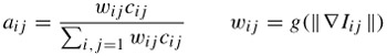 

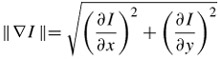
where c_ij is the initial filter coefficient, w_ij is the weight assigned to each coefficient based on the local gradient magnitude ∇I_ij and g is the diffusion function [8]. If w_ij = 1, then the diffusion is linear. The local gradient is computed for all pixels within the kernel by taking the difference between the centre and the corresponding pixels. More precisely, ∇I_ij = I_ij - I_c, where I_c is the value of the centre pixel and I_ij are the pixels within the filter kernel.

Figure 10.6 shows the diffusion function and the corresponding adapted Gaussian kernel to inhibit diffusion across a step edge. The Figure shows that for large gradient magnitudes, the filter coefficient is reduced in order not to diffuse across edges. Similarly, at the lower gradient magnitudes (well away from the edges) within the area of almost uniform texture, the diffusion is unconstrained, so as to have maximum smoothness. The gradient image generated in this form is suitable to be segmented at its object borders by the watershed transform.

Figure 10.6: Weighting function (left), adapted Gaussian kernel (right)

10.3.3.2 Colour edge detection

Colour often gives more information about the object boundaries than the luminance. However, although gradient detection in greyscale images is to some extent easy, deriving the gradient of colour images is less straightforward due to separation of the image into several colour components. Each pixel in the RGB colour space can be represented by a position vector in the three-dimensional RGB colour cube:

(10.3) 

Likewise, pixels in other colour spaces can be represented in a similar manner. Hence, the problem of detecting edges in a colour image can be redefined as the problem of computing the gradient between vectors in the three-dimensional colour space. Various methods have been proposed for solving the problem of colour image gradient detection and they include component-wise gradient detection and vector gradient.

Component-wise gradient

In this approach, gradient detection is performed separately for each colour channel, followed by the merging of the results. The simplest way is to apply the Prewitt or the Sobel operator separately on each channel and then combine the gradient magnitude using some linear or nonlinear function [10]. For example:

(10.4) 

where ∇I_R, ∇I_G, ∇I_B represent the gradient magnitude computed for each of the colour channels.

Vector gradient

This approach requires the definition of a suitable colour difference metric in the three-dimensional colour space. This metric should be based on human perception of colour difference, such that a large value indicates significant perceived difference, and a small value indicates colour similarity. A metric that is commonly used is the Euclidean distance between two colour vectors. For the n-dimensional colour space, the Euclidean distance between two colour pixels, A and B, is defined as follows:

(10.5)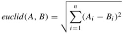 

The gradient of the image is then derived, based on the sum of the colour differences between each pixel and its neighbours. This approximates the Prewitt kernel and is given by the following equations.

(10.6) 

The gradient magnitude is then defined as:

The use of Euclidean distance in the RGB colour space does not give a good indication of the perceived colour differences. Hence, in [9], it was proposed that the vector gradient should be computed in the CIELUV colour space. CIELUV is an approximation of a perceptually uniform colour space, which is designed so that the Euclidean distance could be used to quantify colour similarity or difference [10].

10.3.4 Watershed transform

The watershed transform algorithm can be visualised by adopting a topological view of the image, where high intensity values represent peaks and low intensity values represent valleys. Water is flooded into the valleys and the lines where the waters from different valleys meet are called the watershed lines, as shown in Figure 10.7. The watershed lines separate one region (catchment basin) from another. In actual implementation, all pixels in an image are initially classified as unlabelled and they are examined starting from the lowest intensity value. If the pixel that is currently being examined has no labelled neighbours, it is classified as a new region or a new catchment basin. On the other hand, if the pixel was a neighbour to exactly one labelled region, it would be classified as belonging to that region. However, if the pixel separates two or more regions, it would be labelled as part of the watershed line.

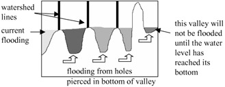
Figure 10.7: Immersion-based watershed flooding

The algorithm can be seeded with a series of markers (seed regions), which represent the lowest point in the image from where water is allowed to start flooding. In other words, these markers form the basic catchment basins for the flooding. In some implementations, new basins are not allowed to form and, hence, the number of regions in the final segmented image will be equal to the number of markers. In other implementations, new regions are allowed to be formed if they are at a higher (intensity) level as compared with the markers. In the absence of markers, the lowest point (lowest intensity value) in the valley is usually chosen as the default marker.

There are two basic approaches to the implementation of the watershed transform and they are the immersion method [11] and the topological distance method [5]. Results obtained using different implementations are usually not identical.

10.3.4.1 Immersion watershed flooding

Efficient implementations of immersion-based watershed flooding are largely based on Vincent and Soille's algorithm [11]. Immersion flooding can be visualised by imagining that holes are pierced at the bottom of the lowest point in each valley. The image is then immersed in water, which flows into the valley from the holes. Obviously, the lowest intensity valley will get flooded first before valleys that have a higher minimum point, as shown in Figure 10.7.

Vincent and Soille's algorithm uses a sorted queue in which pixels in the image are sorted based on their intensity level. In this way, pixels of low intensity (lowest points in valleys) could be examined first before the higher intensity pixels. This algorithm achieves fast performance since the image is scanned in its entirety only once during the queue setup phase.

10.3.4.2 Topological distance watershed

In the topological distance approach, a drop of water that falls on the topology will flow to the lowest point via the slope of the steepest descent. The slope of the steepest descent is loosely defined as the shortest distance from the current position to the local minima. If a certain point in the image has more than one possible steepest descent, that point would be a potential watershed line that separates two or more regions. A more rigorous mathematical definition of this approach can be found in [5].

10.3.5 Colour similarity merging

Despite the use of nonlinear diffusion and the colour gradient, the watershed transformation algorithm still produces an excessive number of regions. For this reason, the regions must be merged based on colour similarity in a suitable colour space. The CIELUV uniform colour space is a plausible candidate due to the simplicity of quantifying colour similarity based on Euclidean distances. The mean luminance L and colour differences u* and v* values are computed for each region of the watershed transformed image. The regions are examined in the increasing order of size and merged with their neighbours if the colour difference between them is less than a threshold (T_h). More precisely, the regions A and B are merged if:

(10.7) 

where A_L,u*,_v* and B_L,u*,v* are the mean CIELUV values of the respective regions. Since it is likely that each region would have multiple neighbours, the neighbour that minimises the Euclidean distance is chosen as the target for merging. After each merging, the mean L, u* and v* values of the merged region are updated accordingly.

10.3.6 Region motion estimation

Spatial segmentation alone cannot discriminate the foreground objects in a video sequence. Motion information between the current frame and a future reference frame must be utilised to identify the moving regions of the image. These moving regions can then be classified as foreground objects or as regions of interest.

Motion estimation is performed for each of the regions after the merging process. Since regions can have any arbitrary shapes, the boundary of each region is extended to its tightest fitting rectangle. Using the conventional block matching motion estimation algorithm (BMA), the motion of the fitted rectangular is estimated.

Figure 10.8 gives a pictorial summary of the whole video segmentation process. The first frame of the video after filtering and gradient operator generates the gradient of the diffused image. This image is then watershed transformed into various regions, some of which might be similar in colour and intensity. In the above example, the watershed transformed image has about 2660 regions, but many regions are identical in colour. Through the colour similarity process, identical colour regions are merged into about 60 regions (in this picture). Finally, homogeneous neighbouring regions are grouped together, and are separated from the static background, resulting in two objects: the ball and the hand and the table tennis racket.

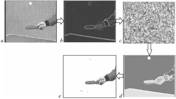
Figure 10.8: A pictorial representation of video segmentation (a original) (b gradient) (c watershed transformed) (d colour merged) (e segmented image)

10.3.7 Object mask creation

The final step of the segmentation process is the creation of the object mask. The object mask is synonymous with object segmentation, since it is used to extract the object from the image. The mask can be created from the union of all regions that have nonzero motion vectors. This works well for sequences that have a stationary background with a single moving object. For more complex scenes with nonstationary background and multiple moving objects, nine object masks are created for the image. Each mask is the union of all regions with coherent motion. Mask 0 corresponds to regions of zero motion, and the other eight masks are regions with motion in the N, NE, E, SE, S, SW, W and NW directions, respectively. These object masks are then used to extract the foreground objects from the video frame.

Figure 10.9 shows two examples of creating the object mask and extracting the object, for two video sequences. The mother and daughter sequence has a fairly stationary background and hence the motion information, in particular motion over several frames, can easily separate foreground from the background.

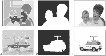
Figure 10.9: (a gradient image) (b object mask) (c segmented object)

For the BBC car, due to the camera following the car, the background is not static. Here before estimating the motion of the car, the global motion of the background needs to be compensated. In section 10.7 we will discuss global motion estimation.

The contour or shape information for each object can also be derived from the object masks and used for tracking the object through the video sequence. Once the object is extracted and its shape is defined, the shape information has to be coded and sent along with the other visual information to the decoder. In the following section several methods for coding of shapes are presented.