3.1 Spatial redundancy reduction
3.1 Spatial redundancy reduction
3.1.1 Predictive coding
In the early days of image compression, both signal processing tools and storage devices were scarce resources. At the time, a simple method for redundancy reduction was to predict the value of pixels based on the values previously coded, and code the prediction error. This method is called differential pulse code modulation (DPCM). Figure 3.1 shows a block diagram of a DPCM codec, where the differences between the incoming pixels from the predictions in the predictor are quantised and coded for transmission. At the decoder the received error signal is added to the prediction to reconstruct the signal. If the quantiser is not used it is called lossless coding, and the compression relies on the entropy coder, which will be explained later.
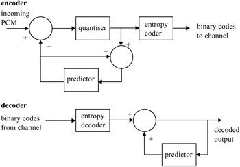
Figure 3.1: Block diagram of a DPCM codec
Best predictions are those from the neighbouring pixels, either from the same frame or pixels from the previous frame, or their combinations. The former is called intraframe predictive coding and the latter is interframe predictive coding. Their combination is called hybrid predictive coding.
It should be noted that, no matter what prediction method is used, every pixel is predictively coded. The minimum number of bits that can be assigned to each prediction error is one bit. Hence, this type of coding is not suitable for low bit rate video coding. Lower bit rates can be achieved if a group of pixels are coded together, such that the average bit per pixel can be less than one bit. Block transform coding is most suitable for this purpose, but despite this DPCM is still used in video compression. For example, interframe DPCM has lower coding latency than interframe block coding. Also, DPCM might be used in coding of motion vectors, or block addresses. If motion vectors in a moving object move in the same direction, coding of their differences will reduce the motion vector information. Of course, the coding would be lossless.
3.1.2 Transform coding
Transform domain coding is mainly used to remove the spatial redundancies in images by mapping the pixels into a transform domain prior to data reduction. The strength of transform coding in achieving data compression is that the image energy of most natural scenes is mainly concentrated in the low frequency region, and hence into a few transform coefficients. These coefficients can then be quantised with the aim of discarding insignificant coefficients, without significantly affecting the reconstructed image quality. This quantisation process is, however, lossy in that the original values cannot be retained.
To see how transform coding can lead to data compression, consider joint occurrences of two pixels as shown in Figure 3.2.
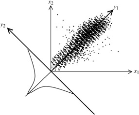
Figure 3.2: Joint occurrences of a pair of pixels
Although each pixel x1 or x2 may take any value uniformly between 0 (black) to its maximum value 255 (white), since there is a high correlation (similarity) between them, then it is most likely that their joint occurrences lie mainly on a 45 degrees line, as shown in the Figure. Now if we rotate the x1x2 coordinates by 45 degrees, to a new position y1y2, then the joint occurrences on the new coordinates have a uniform distribution along the y1 axes, but are highly peaked around zero on the y2 axes. Certainly, the bits required to represent the new parameter y1 can be as large as any of x1 or x2, but that of the other parameter y2 is much less. Hence, on average, y1 and y2 can be represented at a lower bit rate than x1 and x2.
Rotation of x1x2 coordinates by 45 degrees is a transformation of vector [x1, x2] by a transformation matrix T:
| (3.1) | 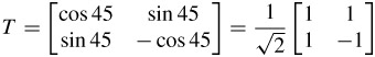 |
Thus, in this example the transform coefficients [y1, y2] become:
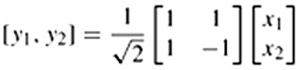
or
| (3.2) | 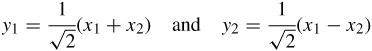 |
y1 is called the average or DC value of x1 and x2 and y2 represents their residual differences. The normalisation factor of ![]() makes sure that the signal energy due to transformation is not changed (Parseval theorem). This means that the signal energy in the pixel domain,
makes sure that the signal energy due to transformation is not changed (Parseval theorem). This means that the signal energy in the pixel domain, ![]() , is equal to the signal energy in the transform domain,
, is equal to the signal energy in the transform domain, ![]() . Hence the transformation matrix is orthonormal.
. Hence the transformation matrix is orthonormal.
Now, if instead of two pixels we take N correlated pixels, then by transforming the coordinates such that y1 lies on the main diagonal of the sphere, then only the y1 coefficient becomes significant, and the remaining N - 1 coefficients, y2, y3,...,yN, only carry the residual information. Thus, compared with the two pixels case, larger dimensions of transformation can lead to higher compression. Exactly how large the dimensions should be depends on how far pixels can still be correlated to each other. Also, the elements of the transformation matrix, called the basis vectors, have an important role on the compression efficiency. They should be such that only one of the transform coefficients, or at most a few of them, becomes significant and the remaining ones are small.
An ideal choice for the transformation matrix is the one that completely decorrelates the transform coefficients. Thus, if Rxx is the covariance matrix of the input source (pixels), x, then the elements of the transformation matrix T are calculated such that the covariance of the coefficients Ryy = TRxxTT is a diagonal matrix (zero off diagonal elements). A transform that is derived on this basis is the well known Karhunen-Loève transform (KLT) [1]. However, although this transform is optimum, and hence it can give the maximum compression efficiency, it is not suitable for image compression. This is because, as the image statistics change, the elements of the transform need to be recalculated. Thus, in addition to extra computational complexity, these elements need to be transmitted to the decoder. The extra overhead involved in the transmission significantly restricts the overall compression efficiency. Despite this, the KLT is still useful and can be used as a benchmark for evaluating the compression efficiency of other transforms.
A better choice for the transformation matrix is that of the discrete cosine transform (DCT). The reason for this is that it has well defined (fixed) and smoothly varying basis vectors which resemble the intensity variations of most natural images, such that image energy is matched to a few coefficients. For this reason its rate distortion performance closely follows that of the Karhunen-Loève transform, and results in almost identical compression gain [1]. Equally important is the availability of efficient fast DCT transformation algorithms that can be used, especially, in software-based image coding applications [2].
Since in natural image sequences pixels are correlated in the horizontal and vertical directions as well as in the temporal direction of the image sequence, a natural choice for the DCT is a three-dimensional one. However, any transformation in the temporal domain requires storage of several picture frames, introducing a long delay, which restricts application of transform coding in telecommunications. Hence transformation is confined to two dimensions.
A two-dimensional DCT is a separable process that is implemented using two one-dimensional DCTs: one in the horizontal direction followed by one in the vertical. For a block of M × N pixels, the forward one-dimensional transform of N pixels is given by:
| (3.3) |
where
C(u) = ![]() for u = 0
for u = 0
C(u) = 1 otherwise
f(x) represents the intensity of the xth pixel, and F(u) represents the N one-dimensional transform coefficients. The inverse one-dimensional transform is thus defined as:
| (3.4) |
Note that the ![]() normalisation factor is used to make the transformation ortho-normal. That is, the energy in both pixel and transform domains is to be equal. In the standard codecs the normalisation factor for the two-dimensional DCT is defined as
normalisation factor is used to make the transformation ortho-normal. That is, the energy in both pixel and transform domains is to be equal. In the standard codecs the normalisation factor for the two-dimensional DCT is defined as ![]() . This gives DCT coefficients in the range of -2047 to +2047. The normalisation factor in the pixel domain is then adjusted accordingly (e.g. it becomes 2/N).
. This gives DCT coefficients in the range of -2047 to +2047. The normalisation factor in the pixel domain is then adjusted accordingly (e.g. it becomes 2/N).
To derive the final two-dimensional transform coefficients, N sets of one-dimensional transforms of length M are taken over the one-dimensional transform coefficients of similar frequency in the vertical direction:
| (3.5) |
where C(v) is defined similarly to C(u).
Thus a block of MN pixels is transformed into MN coefficients. The F(0, 0) coefficient represents the DC value of the block. Coefficient F(0, 1), which is the DC value of all the first one-dimensional AC coefficients, represents the first AC coefficient in the horizontal direction of the block. Similarly, F(1, 0), which is the first AC coefficient of all one-dimensional DC values, represents the first AC coefficient in the vertical direction, and so on.
In practice M = N = 8, such that a two-dimensional transform of 8 x 8 = 64 pixels results in 64 transform coefficients. The choice of such a block size is a compromise between the compression efficiency and the blocking artefacts of coarsely quantised coefficients. Although larger block sizes have good compression efficiency, the blocking artefacts are subjectively very annoying. At the early stage of standardisation of video codecs, the block sizes were made optional at 4 × 4, 8 × 8 and 16 × 16. Now the block size in the standard codecs is 8 × 8.
3.1.3 Mismatch control
Implementation of both forward and inverse transforms (e.g. eqns 3.3 and 3.4) requires that the cos elements be approximated with finite numbers. Due to this approximation the reconstructed signal, even without any quantisation, cannot be an exact replica of the input signal to the forward transform. For image and video coding applications this mismatch needs to be controlled, otherwise the accumulated error due to approximation can grow out of control resulting in an annoying picture artefact.
One way of preventing error accumulation is to let the error oscillate between two small levels. This guarantees that the accumulated error never exceeds its limit. The approach taken in the standard codecs is to say (e.g. MPEG-2), at the decoder, that the sum of all the values of the 8 × 8 = 64 transform coefficients should be an odd number (no matter whether they are quantised or not). In case the sum is an even number, the value of the highest frequency coefficient, F(7, 7), is either incremented or decremented by 1, depending whether its value itself is odd or even, respectively. This, of course, introduces a very small error, but it cannot be noticed on images for two reasons. First, at the inverse transform, the reconstructed pixels are divided by a large value of the order of N2. Second, since error is introduced by the highest frequency coefficient, it appears as a very high frequency, small amplitude dither-like noise, which is not perceivable at all (the human eye is very tolerant to high frequency noise).
3.1.4 Fast DCT transform
To calculate transform coefficients, every one-dimensional forward or inverse transformation requires eight multiplications and seven additions. This process is repeated for 64 coefficients, both in the horizontal and vertical directions. Since software-based video compression is highly desirable, methods of reducing such a huge computational burden are also highly desirable.
The fact that DCT is a type of discrete Fourier transform, with the advantage of all-real coefficients, means that one can use a fast transform, similar to the fast Fourier transform, to calculate transform coefficients with complexity proportional to N log2 N, rather than N2. Figure 3.3 shows a butterfly representation of the fast DCT [2]. Intermediate nodes share some of the computational burden, hence reducing the overall complexity. In the Figure, p[0]-p[7] are the inputs to the forward DCT and b[0]-b[7] are the transform coefficients. The inputs can be either the eight pixels for the source image, or eight transform coefficients of the first stage of the one-dimensional transform. Similarly, for inverse transformation, b[0]-b[7] are the inputs to the IDCT, and p[0]-p[7] are the outputs. A C language programme for fast forward DCT is given in Appendix A. In this program, some modifications to the butterfly matrices are made to trade-off the number of additions for multiplications, since multiplications are more computationally intensive than additions. A similar program can be written for the inverse transform.
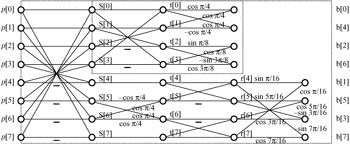
Figure 3.3: A fast DCT flow chart
EAN: 2147483647
Pages: 148