Capacity Planning for the Processor | Microsoft SQL Server 2000 Administrators Companion

3 4

Now that we have sized and analyzed the memory, it's time to do the same for the processor. At this point, we can make the following assumptions about the system:

The application and database design schema is complete.
The target steady state CPU utilization is less than 75 percent.
Expected cache hit rate is at least 90 percent.
No disk drive will exceed 85 percent usage of space or I/O activity.
The server is running only a database.
Distribution of disk I/Os is even across all drives.

We've made use of these assumptions as guidelines and thresholds for sizing memory, but for anticipating capacity for the CPU, we need additional information. This information can be provided by the database designer and the application designer.

Anticipating the capacity of a CPU on a database server is not as complicated as you might think. Remember that a database server is only processing transactions. The application is running on a client machine, so application sizing does not enter into the equation. The server will be processing requests from users in the form of read and write operations—that is, it will be processing I/Os. The application designer can provide pertinent information about the nature of the transactions. The database designer can provide information pertaining to the tables and their indexes that will be affected by these transactions. So the task at hand will be to determine how many I/Os will be generated by the transactions and in what time frame they have to be completed. We need to know how many transactions the system will be required to process and the definition of either the working day in terms of hours for this system or the peak utilization period.

As we've seen, it's always preferable to size for the peak utilization period because it represents the worst-case scenario and we can build the machine to accommodate it. Unfortunately, in most cases this information will not be available, so we are forced to use the information we have pertaining to steady state. To gain a deeper understanding of the transactions that we will be processing, we need access to the transaction anatomy, or profile, which will help us determine the numbers of reads and writes (I/Os) that will be generated and enable us to calculate the anticipated CPU utilization. We get this information from our interview with the database designers and the application designers. First we need to know how many transactions of each type will go through the system, and then we need to determine the number of I/Os that will be generated. This calculation will provide an estimate of the CPU workload.

For an existing system, the user can profile transactions by running each of the transactions one at a time and tracking them using Performance Monitor to determine the number of I/Os generated. This "real" information can be used to adjust the speed, type, and number of CPUs in use.

So far, we have talked about sizing the CPU in terms of I/Os generated by user transactions. I/Os can also be generated by the fault tolerance equipment that may be in use. These additional I/Os must also be considered when you are sizing the CPU.

Fault Tolerance

Most computer companies today provide fault tolerance through the support of RAID (Redundant Array of Inexpensive Disks) technology. (See Chapter 5 for an in-depth description of RAID technology.) Remember that the most commonly used RAID levels are as follows:

RAID 0 Single disk drive
RAID 1 Mirrored disk drive
RAID 5 Multiple disk drives and data striping

Because RAID 0 requires a single disk, it has a single point of failure—in other words, if the disk drive fails, you will lose the data on that disk drive and therefore the entire database. A RAID 0 array is shown in Figure 4-1. RAID 1 provides a mirror image of the database disk drive. If a disk drive fails, you have a backup data drive complete with all the data that was on the failed disk drive. If you specify RAID 1, users get the added benefit of split seeks (covered in Chapter 5), which enable the system to search both drives simultaneously, greatly accelerating search speed and thereby reducing your transaction response time. A RAID 1 array is shown in Figure 4-2.

The choice of RAID level directly affects the number of disk I/Os because different RAID levels alter the number of writes to the disk. For example, RAID 1 requires twice as many writes as RAID 0. If the user describes a transaction as having 50 reads and 10 writes and wants to use RAID 1, the number of writes increases to 20.

If a RAID 0 configuration has two designated disk drives, a comparable RAID 5 configuration would have three disk drives. In a RAID 5 configuration, a parity stripe is used that contains information about the data on the other two drives that can be used to rebuild a failed disk's data. A RAID 5 array is shown in Figure 4-4. This database protection scheme comes with a performance cost as well as a dollar cost. Each write under RAID 5 will add twice the number of reads and twice the number of writes for each transaction processed because each transaction must be written to two disks, and the parity stripe must be read, altered to incorporate the new data, and then written. This redundancy will lengthen the transaction response time slightly.

To calculate the number of I/Os for the various RAID levels, you can use the following equations.

For RAID 0:

 number of I/Os = (number of reads per transaction) +                  (number of writes per transaction)

If a transaction has 50 reads and 10 writes, the total number of I/Os using RAID 0 is 60.

For RAID 1:

 number of I/Os = (number of reads per transaction) +                  (2 * (number of writes per transaction))

If a transaction has 50 reads and 10 writes, the total number of I/Os using RAID 1 is 70.

For RAID 5:

 number of I/Os = 3 * (number of I/Os per transaction)

If a transaction has 50 reads and 10 writes, the total number of reads would be 150 and the total number of writes would be 30. The total number of I/Os using RAID 5 is therefore 180.

The increase of I/Os is a function of the disk controller and is transparent to the user, who does not need to make adjustments to the application. Remember that your RAID selection directly affects the number of I/Os that will be processed. This increase of reads and writes should be considered, as it will affect the utilization factors of the CPUs and the quantity of disks chosen during sizing.

Once you have calculated the total number of reads and writes due to user transactions and added the additional I/Os due to the RAID levels you have selected, you have all the information you need to calculate the CPU utilization. The following formula is used to determine the CPU utilization of a proposed system:

CPU utilization = (throughput) * (service time) * 100

Here throughput is the number of I/Os to be processed per second, and service time is the amount of time spent processing a typical I/O transaction. This formula simply states that utilization is the total number of I/Os the system processes per second multiplied by the time it takes to perform each task, multiplied by 100 to get a percentage.

To determine the number of CPUs needed for the system, the following steps should be performed on every transaction that will be processed as part of this workload.

Calculate the total number of reads that will be going through the system by using the following formula:
```
 total reads = (reads per transaction) *               (total number of transactions)
```
Determine how many of these reads will be physical I/Os and how many will be logical I/Os by using the following formulas:
```
 total logical reads = (total reads) * (cache hit rate)  total physical reads = (total reads) - (total logical reads)
```
Convert the total number of each read type to reads per second by using the following formulas:
```
 logical reads/sec = (total logical reads) / (work period)  physical reads/sec = (total physical reads) / (work period)
```
The work period should be the length of time, in seconds, in which the work is to be performed.
Calculate the amount of CPU time that was used for each of the read functions by using the following formulas:
```
 logical read time = (logical reads/sec) * (logical read time)  physical read time = (physical reads/sec) * (physical read time)
```
The logical read time is the time it takes to process a logical read. The physical read time is the time it takes to process a physical read. These read times can be obtained using Performance Monitor. (See the sidebar "Obtaining Read Times" at the end of this list for directions.)

NOTE
Typical values for read times are 0.002 second for the physical read time variable and 0.001 second for the logical read time variable.
Calculate the CPU utilization for the various read functions using the following equation:
```
 utilization = (throughput) * (service time) * 100
```
You can break this down into logical and physical read utilization as follows:
```
 logical read utilization = (logical reads/sec) * (logical read time)  physical read utilization = (physical reads/sec) * (physical read time)
```
This information can be used to determine whether there is too much physical read utilization. You can then adjust the cache size so that you will have more logical reads.
Calculate the total number of writes that will be going through the system by using the following formula, where the RAID factor is the total number of expected writes that your workload will perform during the processing period:
```
 total writes = (writes per transaction) * (total number transactions) *                (RAID factor increase)
```
Now find the number of writes per second that will be passing through the system by performing the following calculation:
```
writes/sec = (total writes) / (work period)
```
Again, the work period should be the length of time, in seconds, in which the work is to be performed.
Determine the total CPU time that was used to process the writes by performing the following calculation:
```
CPU write time = (writes/sec) * (CPU write time)
```
Calculate the write utilization by using the following formula:
```
write utilization = (writes/sec) * (CPU write time) * 100
```
Calculate the total CPU utilization for the transaction type by using the following formula:
```
 CPU utilization = ((logical read utilization) + (physical read utilization) +                    (write utilization)) * 100
```
This calculation must be performed for each type of transaction that your system allows. For example, if you have a banking system, you might allow withdrawals, deposits, and balance inquiries. You must perform these utilization calculations separately for each of these three types of transactions to accurately size the CPUs for your system.
Finally, calculate the total processor utilization by using the following formula:
```
total CPU utilization = sum of all transaction utilizations
```

If the total CPU utilization is over the 75 percent threshold, you should add more CPUs to your system. Additional CPUs will reduce the total CPU utilization according to the following formula:

 total CPU utilization (>1 CPU) = (total CPU utilization) /                        (number of CPUs)

Add enough CPUs to bring the total CPU utilization below 75 percent. For example, if total CPU utilization is 180 percent, you would use three CPUs. The resulting total CPU utilization would then be 60 percent for the three-CPU system.

NOTE
You might be wondering why we have not used processor speed in any of our calculations. In fact, we have—indirectly. Processor speed is accounted for in the service time—the amount of time spent processing a transaction.

Obtaining Read Times

You can obtain the read times for your system through Performance Monitor. Turn on Diskperf by entering the following command in an MS-DOS window:

diskperf -y

Next start Performance Monitor, and look in the Physical Disk object for the Avg. Disk sec/Read and Avg. Disk sec/Write counters. Note that these counters give you the average read times for physical reads. Don't worry about these times for logical reads.

Collecting Usage Data for a Single CPU

When your system is implemented, you will need to track CPU usage much as you tracked memory usage. Performance Monitor contains many counters related to individual CPU usage. These counters are contained in the Processor object. The following counters will be the most useful for sizing purposes:

% Processor Time The percentage of the elapsed time that a processor is busy executing instructions. An instruction is the basic unit of execution in a computer, a thread is the object that executes instructions, and a process is the object created when a program is run. This counter can be interpreted as the fraction of time spent doing useful work.
% Privileged Time Percentage of processor time spent in Privileged mode. The Windows NT service layer, the Executive routines, and the Windows NT Kernel all execute in Privileged mode; device drivers for most devices other than graphics adapters and printers also execute in Privileged mode.
% User Time Percentage of processor time spent in User mode. All application code and subsystem code executes in User mode. The graphics engine, graphics device drivers, printer device drivers, and the Window Manager also execute in User mode. Code executing in User mode cannot damage the integrity of the Windows NT Executive, Kernel, or device drivers.
% Interrupt Time Percentage of elapsed time spent by the processor handling hardware interrupts. Interrupts are executed in Privileged mode, so interrupt time is a component of % Privileged Time. This counter can help determine the source of excessive time being spent in Privileged mode.
Interrupts/sec This counter contains the average number of device interrupts the processor experiences per second. A device interrupts the processor when it has completed a task or when it otherwise requires attention. Devices that may generate interrupts include the system timer, the mouse, data communication lines, network interface cards, and other peripheral devices. Normal thread execution is suspended during interrupts, and an interrupt may cause the processor to switch to another, higher priority thread. Clock interrupts are frequent and periodic and create a background of interrupt activity.

Not all of these counters are required to conduct a capacity planning study—the counters you select will be determined by the depth of the study you are conducting. At the very least, the % Processor Time counter should be used.

Collecting Usage Data for Multiple CPUs

You can also retrieve system-averaged data for multiple CPUs via Performance Monitor. Use the System object, which includes the following counters, among others:

% Total Processor Time Sum of the % Processor Times for each processor divided by the number of processors in the system.
% Total Privileged Time Sum of the % Privileged Times for each processor divided by the number of processors in the system.
% Total User Time Sum of the % User Times for each processor divided by the number of processors in the system.
% Total Interrupt Time Sum of the % Interrupt Times for each processor divided by the number of processors in the system.
Total Interrupts/sec Average number of device interrupts that the processors experience per second. This counter provides an indication of how busy system devices are on a computer-wide basis.

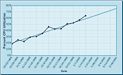
Analyzing CPU Data

The data you obtain using these counters can be used to predict rises in a specific CPU's utilization and therefore increased response times from that CPU. Figure 66 shows CPU utilization over time. Notice that the utilization trend for the CPU is rising; it will reach the 75 percent threshold by February 18, 2000.

click to view at full size.

Figure 6-6. Linear CPU utilization predictive analysis.

NOTE
The more data points you collect, the more accurate your prediction.