Principles of Capacity Planning
3 4
When you cannot define the peak utilization period, pre-capacity planning is usually accomplished by estimating the transaction activity expected during steady state processing.
NOTE
"Steady state" refers to the expected utilization of CPU during the course of your working day. For example, if you expect a CPU utilization of 55 percent during the course of the day, that is steady state. If during that same day, your system experiences a utilization of 90 percent for one hour, that is the peak utilization period.
Once you know the maximum number of transactions you expect to complete in a processing day and the length of your processing day, you can calculate the average number of transactions per unit of time. However, since you don't know the actual rate at which the transactions will occur, you should size your system with a built-in reserve capacity. Reserve capacity refers to a certain portion of system processing power left in reserve to accommodate the more stressed workload periods.
Post-capacity planning on an order entry system involves the constant monitoring of key performance counters to record what the system has done in the past and what it is doing currently. This information is usually stored in a database and is used in general reporting of the performance, capacity consumption, and available reserve capacity. A database application such as Microsoft Excel can be used to generate graphs, spreadsheets, and transaction activity reports, which can be used to predict the machine's resource use.
CPU Utilization
Another reason to build and maintain a machine with reserve capacity relates to the "knee of the curve" theory. Simply stated, this theory predicts that utilization has a direct effect on queues, and because queue lengths are directly related to response time (in fact, queue length is part of the response time equation), utilization has a direct effect on response time. The knee of the curve is the point at which factors like response time and queue length switch from linear growth to exponential growth or the point at which they begin growing asymptotically (to infinity).
REAL WORLD Utilization and Response Times at the Supermarket
Say you go to the supermarket at 3:00 AM, pick up the items you need, and carry them to the checkout counter. At this time in the morning, no one is in line in front of you, so the utilization of that cashier is 0 percent and the queue length (number of people in front of you) is also 0. Your response time will be equal to your service time. This means that your service time—in this case, the time it takes to complete the transaction of tallying your purchases and paying the bill—is all the time it will take to complete this task.Imagine the same scenario at 5:00 PM, a much busier time for a supermarket. Now when you arrive at the checkout counter, eight people are in line in front of you (that is, the queue length is 8). Your response time now is equal to the sum of the individual service times for all eight people ahead of you (which will vary depending on the number of items they are purchasing, whether they are paying by check or with cash, and so on), plus your own service time. The utilization of the cashier is also much higher at 5:00 PM than at 3:00 AM, which has a direct effect on the length of the queue and therefore on your overall response time.
Linear Growth vs. Exponential Growth
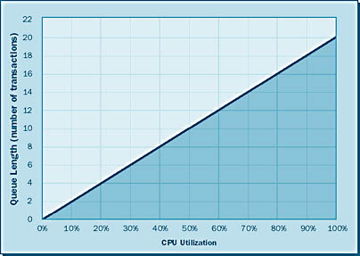
Normally, we try to keep a system running linearly—that is, so that the growth of the queue will be linear. As illustrated in Figure 6-1, linear growth is the even, incremental growth of queues in relation to utilization growth. The rule of thumb is that as long as CPU utilization remains below 75 percent, queue growth will remain linear.
Sometimes, however, a CPU is utilized in a steady state of above 75 percent. This scenario has certain drawbacks—in particular, this high utilization causes exponential growth of queue lengths. Exponential growth is geometrically increasing growth, as shown in Figure 6-2.
NOTE
For the figures in this chapter, the service time of a transaction has been set to 0.52 second, and every transaction is assumed to have the same service time.
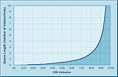
Notice that at about 75 percent CPU utilization, the queue length curve shifts from linear growth to exponential growth (that is, the curve becomes an almost vertical line).
Response Time
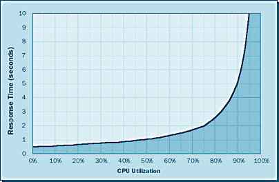
The graph in Figure 6-3 illustrates how utilization has a direct effect on the response times. Notice that similar curves occur in the response time graph and the queue length graph. The dramatic increase in response times shown in both graphs demonstrates why you never want to run your CPUs in a steady state of over 75 percent utilization. This is not to say that you can never run your CPUs above 75 percent, but the longer you do so, the more negative impact you will experience in terms of queue length and response time. Not exceeding the knee of the curve—in this case, 75 percent utilization—is one of the most important principles of sizing and should be considered when you are determining the number of CPUs your sys-tem will require. For example, suppose you are sizing a system that you calculate will produce an anticipated total processor utilization factor of 180 percent. You could endure the horrendous performance of such a system, or you could run two CPUs at 90 percent utilization—15 percentage points above the knee of the curve. It would be better, however, to run three CPUs at about 60 percent, keeping the utilization 15 percentage points below the knee of the curve.
This principle also applies to other elements of your system, such as disks. Disks do not have the same knee of the curve as processors do—the knee of the curve for disks tends to occur at 85 percent utilization. This 85 percent threshold applies to both the size and I/O capability of the disk drive. For example, a 9-GB disk should not contain more than 7.65 GB of data stored at any given time. This data limit will allow for growth, but more important it will help keep down response time because a disk at full capacity will have longer seek times, adding to the overall response time. By the same principle, if a disk drive has an I/O capability of 70 I/Os per second, you would not want to have a constant I/O arrival rate of more than 60 I/Os per second in a steady state of operation. By following this principle, you can minimize your overall response times and get the most out of your system because you will not be using your processors or disks at maximum utilization. Your system will also retain a reserve capacity for peak utilization periods.
NOTE
Remember that for optimal performance, keep your CPU utilization below 75 percent and your disk utilization below 85 percent.
Page Faulting
Not exceeding the knee of the curve is an important principle for sizing processors and disks, but what about memory? To help size memory, we use the principle of page faulting. Page faults are a normal system function and are used to retrieve data from the disk. If the system needs a certain code or data page and that page exists in memory, a logical I/O event occurs, meaning that the code or data is read from memory and the transaction that needed the code or data is processed.
But what if the needed code or data page is not in memory? In that case, we must perform a physical I/O to read the needed page from the disk. This task is accomplished via page faulting. The system will issue a page fault interrupt when a needed code or data page is not in its working set in main memory. The page fault instructs another part of the system to retrieve the code or data from the physical disk—in other words, if the code or data page your system is seeking is not in memory, the system will issue a page fault to instruct another part of the system to perform a physical I/O and go to the disk to retrieve it. A page fault will not cause the page to be retrieved from the disk if that page is on the standby list, and hence already in main memory, or if it is in use by another process with which the page is shared.
There are two types of physical I/Os: user and system. A user physical I/O occurs when a user transaction asks to read data that is not found in memory. A simple data transfer from the disk to memory occurs. This transfer is usually handled by some sort of data flow manager combined with disk controller functions. A system physical I/O occurs when the system requires a code page for a process it is running and the code page is not in memory. The system issues a page fault interrupt, which prevents processing until the required data has been retrieved from disk. After this retrieval, processing continues. Both physical I/O conditions will prolong response time because the retrieval time for data found in memory is rated in microseconds (millionths of seconds) whereas physical I/Os are rated in milliseconds (thousandths of seconds). Since page fault activities cause physical I/Os, which prolong response time, we will achieve better system performance by minimizing page faults.
Three types of page faults can occur in your system:
Operating system page faults If the system is executing operating system code and the next code address is not in memory, the system will issue an operating system page fault interrupt to retrieve the next code address from the disk. For a code address fault, the transfer of the code data goes from the disk to memory, requiring a single physical I/O to complete.
Application code page faults If the system is executing any other code and the next code page is not in memory, the system will issue a page fault interrupt to retrieve the next code page from the disk. For these page faults, the transfer of the code data goes from the disk to memory, requiring a single physical I/O to complete.
Page fault swap In the case of a data page that has been modified (known as a "dirty" page), a two-step page fault known as a page fault swap is used, causing the system not only to retrieve the new data from the disk, but also to write the current data in memory out to the disk. This two-step page fault requires two physical I/Os to complete, but it will ensure that any changed data is saved. If swapping occurs often enough, it can be the single most damaging factor in response time. Remember that page fault transfers occur in whole pages, even if only a few bytes are actually needed. Page fault swaps take more time than page faults because they incur twice as many physical I/Os. For this reason, you should minimize the number of page fault swaps in your system.
When you are estimating the minimum memory requirement for a new system, always try to anticipate the total memory that you will need to process the workload by finding the memory specifications of all processes (including the operating system and database engines) that will run on your system. And don't forget about page faults. To maintain a system's memory, information about page fault activity should be collected and stored as part of the performance database. Predictive analysis should be performed on this data to project when you will require additional memory. A comfortable margin of available memory should be maintained for peak usage. When you are planning a system, try to maintain 5 to 10 percent additional memory over what is required for the processes that will be running.
NOTE
You cannot remove all page faulting from your system, but you can minimize it. You should add memory when you experience more than two page faults per second. Performance monitors (such as the counter for page faults per second) are described in the following section.
EAN: N/A
Pages: 264