2. Techniques

2. Techniques

In order to describe the alternative techniques, we assume a configuration consisting of K disk models: D₀, D₁,..., D_K-1. There are q_i disks belonging to disk model i: ,...,. A disk drive of model D_i consists of m_i zones. To illustrate, Figure 35.2 shows a configuration consisting of two disk models Do and D₁ (K=2). There are two disks of each model (q₀=q₁=2), numbered ,,,. Disks of model 0 consist of 2 zones (m₀=2) while those of model 1 consist of 3 zones (m₁=3). Zone j of a disk (say ) is denoted as Z_j(). Figure 35.2 shows a total of 10 zones for the 4 disk drives and their unique indexes. The k^th physical track of a specific zone is indexed as PT_k(Z_j)).

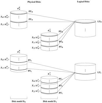
Figure 35.2: OLT1.

We use the set notation, { : }, to refer to a collection of tracks from different zones of several disk drives. This notation specifies a variable before the colon and the properties that each instance of the variable must satisfy after the colon. For example, to refer to the first track from all zones of the disk drives that belong to disk model 0, we write:

With the configuration of Figure 35.2, this would expand to:

2.1 IBM's Logical Track [25]

This section starts with a description of this technique for a single multi-zone disk drive. Subsequently, we introduce two variations of this technique, OLT1 and OLT2, for a heterogeneous collection of disk drives. While OLT1 constructs several logical disks from the physical disks, OLT2 provides the abstraction of only one logical disk. We describe each in turn.

With a single multi-zone disk drive, this technique constructs a logical track from each distinct zone provided by the disk drive. Conceptually, this approach provides equi-sized logical tracks with a single data transfer rate such that one can apply traditional continuous display techniques [2, 27, 3, 13, 21, 23]. With K different disk models, a naive approach would construct a logical track LT_k by utilizing one track from each zone: LT_k = {PT_k(Z_j()):∀i, j, p} where 0 ≤ j < m_i and 0 ≤ i< K and 0 ≤ p < q_i.

With this technique, the value of k is bounded by the zone with the fewest physical tracks, i.e., 0 ≤ k < Min[ NT(Z_j()) ], where NT(Zj()) is the number of physical tracks in zone j of disk model D_i. Large logical tracks result in a significant amount of memory per simultaneous display, rendering a continuous media server economically unavailable. In the next section, we describe two optimized versions of this technique that render its memory requirements reasonable.

2.2 Optimized Logical Track 1 (OLT1)

Assuming that a configuration consists of the same number of disks for each model, ^[5] OLT1 constructs logical disks by grouping one disk from each disk model (q logical disks). For each logical disk, it constructs a logical track consisting of one track from each physical zone of a disk drive. To illustrate, in Figure 35.2, we pair one disk from each model to form a logical disk drive. The two disks that constitute the first logical disk in Figure 35.2, i.e., disks and , consist of a different number of zones ( has 2 zones while has 3 zones). Thus, a logical track consists of 5 physical tracks, one from each zone.

Logical disks appear as a homogeneous collection of disk drives with the same bandwidth. There are a number of well known techniques that can guarantee hiccup-free display given such an abstraction, see [2, 27, 3, 13, 21, 23, 26]. Briefly, given a video clip X, these techniques partition X into equi-sized blocks that are striped across the available logical disks [3, 26, 27]: one block per logical disk in a round-robin manner. A block consists of either one or several logical tracks.

Let T_i denote the time to retrieve m_i tracks from a single disk of model D_i consisting of m_i zones: T_i = m_i (a revolution time + seek time). Then, the transfer rate of a logical track (R_LT) is: R_LT = (size of a logical track)/Max[T_i] for all i, 0 ≤ i < K.

In Figure 35.2, to retrieve a LT from the first logical disk, incurs 2 revolution times and 2 seeks to retrieve two physical tracks, while disk incurs 3 revolutions and 3 seeks to retrieve three physical tracks. Assuming a revolution time of 8.33 milliseconds (7200 rpm) and the average seek time of 10 milliseconds for both disk models, requires 36.66 milliseconds (T₀ = 36.66) while requires 54.99 (T₁ = 54.99) milliseconds to retrieve a LT. Thus, the transfer rate of the LT is determined by disk model D₁. Assuming that a LT is 1 megabyte in size, its transfer rate is (size of a logical track)/Max[T₀,T_I] = 1 megabyte/54.99 milliseconds = 18.19 megabytes per second.

This example demonstrates that OLT1 wastes disk bandwidth by requiring one disk to wait for another to complete its physical track retrievals. In our example, this technique wastes 33.3 % of Do's bandwidth. In addition, this technique wastes disk space because the zone with the fewest physical tracks determines the total number of logical tracks. In particular, this technique eliminates the physical tracks of those zones that have more than NT_min tracks, NT_min=Min[NT(Z_j()) ], i.e., it eliminates PT_k( Z_j() ) that have NT_min ≤ k < NT( Z_j() ), for all i and j, 0 ≤ i<K and 0 ≤ j < m_i.

2.3 Optimized Logical Track 2 (OLT2)

OLT2 extends OLT1 with the following additional assumption: each disk model has the same number of zones, i.e., m_i is identical for all disk models, 0 ≤ i < K. Using this assumption, it constructs logical tracks by pairing physical tracks from zones that belong to different disk drives. This is advantageous for two reasons. First, it eliminates the seeks required per disk drive to retrieve the physical tracks. Second, assuming an identical revolution rate of all heterogeneous disks, it prevents one disk drive to wait for another.

The details of OLT2 are as follows. First, it reduces the number of zones of each disk to that of the disk with fewest zones: m_min = Min[m_i] for all i, 0 ≤ i < K. Hence, we are considering only zones, Z_j() for all i, j, and k (0 ≤ i < K, 0 ≤ j < m_min, and 0 ≤ k < q). For example, in Figure 35.3, the slowest zone of disks of and (Z₂)are eliminated such that all disks utilize only two zones. This technique requires m_min disks of each disk model (totally m_min K disks). Next, it constructs LTs such that no two physical tracks (from two different zones) in a LT belong to one physical disk drive. A logical track LT_k consists of a set of physical tracks:

(35.1)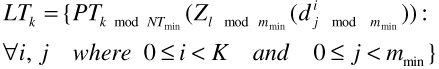

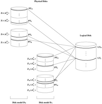
Figure 35.3: OLT2.

where . The total number of LTs is m_min NT_min, thus 0 ≤ k < m_min NT_min.

OLT2 may use several possible techniques to force all disks to have the same number of zones. For each disk with δ_Z zones more than m_min, it can either (a) merge two of its physically adjacent zones into one, repeatedly, until its number of logical zones is reduced to m_min, (b) eliminate its innermost δ_Z zones, or (c) a combination of (a) and (b). With (a), the number of simultaneous displays is reduced because the bandwidth of two merged zones is reduced to the bandwidth of the slower participating zone. With (b), OLT2 wastes disk space while increasing the average transfer rate of the disk drive, i.e., number of simultaneous displays. In [11], we describe a configuration planner that empowers a system administrator to strike a compromise between these two factors for one of the techniques described in this study (HetFIXB). The extensions of this planner in support of OLT2 is a part of our future research direction.

^[5]This technique is applicable as long as the number of disks for each model is a multiple of the model with the fewest disk drives: if min(q_i), 0 ≤ i < K, denotes the model with fewest disks, then q_j is a multiple of min(q_i).