3. Camera Motion Compensation

3. Camera Motion Compensation

If videos are recorded with a moving camera, not only the foreground objects are moving, but also the background. The first step of our segmentation algorithm determines the motion due to changes in the camera parameters. This allows to stabilize the background such that only the foreground objects are moving relative to the coordinate system of the reconstructed background. It is usually assumed that the background motion is the dominant motion in the sequence, i.e., its area of support is much larger than the foreground objects.

In order to differentiate between foreground and background motion, one has to introduce a regularization model for the motion field. This model should be general enough to describe all types of motion that can occur for a single object, but on the other hand, it should be sufficiently restrictive that two motions that we consider "different" can not be described by the same model. The motion model also allows to determine motion in areas in which the texture content is not sufficient to estimate the correct motion.

3.1 Camera Motion Models

We use a world model in which the image background is planar and non-deformable. This assumption, which is valid for most practical sequences, allows us to use a much simpler motion model as would be needed for the general case of a full three-dimensional structure.

Using homogeneous coordinates, the projection of a 3D scene to an image plane can be formulated in the most general case by (x' y' w)^T = P (x y z 1)^T, where P is a 3 4 matrix (see [3,6,7]). As we are only interested in the transformation of one projected image to another projected image at a different camera position (c.f. Fig. 23.2), we can arbitrarily change the world coordinate system such that the background plane is located at z = 0. In this case, the projection equation reduces to

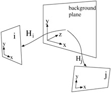
Figure 23.2: Projection of background plane in world coordinates to image coordinate systems of images i and j.

(23.1)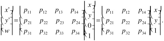

The 3 3 matrix on the right denotes a plane-to-plane mapping (homography). Let H_i be the homography to project the background plane onto the image plane of frame i. Then, we can determine the transformation from image plane i to j as

(23.2)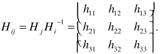

Since homogeneous coordinates are scaling invariant, we can set h'_ij = h_ij / h₃₃ and get with a renaming of matrix elements

(23.3)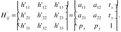

Hence, the transformation between image frames can be written as

(23.4)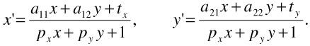

This model is called the perspective camera motion model. In this formulation, it is easy to see that the a_ij correspond to an affine transformation, t_x, t_y are the translatorial components, and p_x, p_y are the perspective parameters. A disadvantage of the perspective motion model, which will become apparent in the next section, is that the model is non-linear. If the viewing direction does not change much between successive frames, the perspective parameters p_x, p_y can be neglected and can be set to zero. This results in the affine camera motion model

(23.5)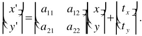

Since the affine model is linear, the parameters can be estimated easily. The selection of the appropriate camera model depends on the application area. While it is possible to use the most general model in all situations, it may be advantageous to restrict to a simpler model. A simple motion model is not only easier to implement, but the estimation also converges faster and is more robust than a model with more parameters. In some applications, it may even be possible to restrict the affine model further to the translatorial model. Here, (a_ij) equals the identity matrix and only the translatorial components t_x, t_y remain:

(23.6)

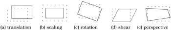
Figure 23.3: Different plane transformations. While transformations (a)-(d) are affine, perspective deformations (e) can only be modeled by the perspective motion model.

3.2 Model Parameter Estimation

In parameter estimation, we search for the camera model parameters that best describe the measured local motion. Algorithms for camera model parameter estimation can be coarsely divided into two classes: feature-based estimation [22] and direct (or gradient-based) estimation [8]. The idea of model estimation based on feature correspondences is to identify a set of positions in the image that can be tracked through the sequence. The camera model is then calculated as the best fit model to these correspondences. In direct matching, the best model parameters are defined as those resulting in the difference frame with minimum energy. This approach is usually solved by a gradient descent algorithm. Hence, it is important to have a good initial estimate of the camera model to prevent getting trapped in a local minimum. As the probability for running into a local minimum increases with large displacements, a pyramid approach is often used. The image is scaled down several levels and the estimation begins at the lowest resolution level. After convergence, the estimation continues at the next higher resolution level until the parameters for the original resolution are found.

Since direct methods provide a higher estimation accuracy than feature-based approaches, but require a good initialization to assure convergence, we are using a two-step process. First, feature-based estimation which can cope with large displacements is used to obtain an initial estimate. Based on this model, a direct method is used to increase the accuracy.

3.3 Feature-Based Estimation

Feature-based estimation is based on a set of features in the image that can be tracked reliably through the sequence. If features can be well localized, image motion can be estimated with high confidence. On the other hand, for pixels inside a uniformly colored region, we cannot determine the correct object motion. Even for pixels that lie on object edges, only the motion component perpendicular to the edge can be determined (see Figure 23.4a). To be able to track a feature reliably, it is required that the neighborhood of the feature shows a structure that is truly two-dimensional. This is the case at corners of regions, or points where several regions overlap (see Figure 23.4b–d).

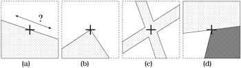
Figure 23.4: Feature points on edges (a) cannot be tracked reliably because a high uncertainty about the position along the edge remains. Feature points at corners (b), crossings (c), or points where several regions overlap (d) can be tracked very reliably.

3.3.1 Feature Point Selection

For the selection of feature points, we employ the Harris (or Plessey) corner detector [5] which is described in the following. Let P = {p_i} be the set of pixels in an image with associated brightness function I(p). To analyze the structure at pixel p = (x_p y_p) ∈ I, a small neighborhood N(p) ⊂ I around p is considered. We denote the image gradient at p as ∇I(p) = (g_x(p) g_y (p))^T. Let us examine how the distribution of gradients has to look like for feature point candidates. Figure 23.5 depicts scatter-plots of the gradient vector components for all pixels inside the neighborhood of some selected image positions. We can see in Figure 23.5c that for neighborhoods that only exhibit one-dimensional structure, the gradients are mainly oriented into the same direction. Consequently, the variance is large perpendicular to the edge and very small along the edge. This small variance indicates that the feature cannot be well localized. Favorably, features should expose a neighborhood where the gradient components are well scattered over the plane and, thus, the variance in both directions is high (cf. Figure 23.5d,e).

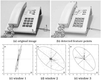
Figure 23.5: Scatter plots of gradient components for a selected set of windows.

Approximating a bivariate Gaussian distribution, we determine the principal axes of the distribution by using a principal component decomposition of the correlation matrix

(23.7)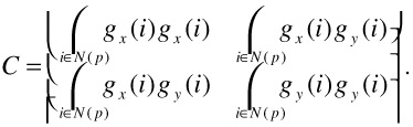

The length of the principal axes corresponds to the eigenvalues λ₁ ≤ λ₂ of C. Based on these eigenvalues, we can introduce a classification of the pixel p. We differentiate between the classes flat for low λ₁, λ₂, edge for λ₁ << λ₂, or corner, textured for large λ₁,λ₂. Since the computation of eigenvalues is computationally expensive (note that the computation has to be performed for every pixel in the image), Harris and Stephens proposed to set the classification boundaries such that an explicit computation of the eigenvalues is not required.

Exploiting the fact that λ₁ + λ₂ = Tr(C) and λ₁ λ₂ = Det(C), they defined a corner response value as

(23.8)

where k is usually set to 0.06. The class boundaries are chosen as shown in Figure 23.6. After r(x,y) has been computed for each pixel, feature points are obtained from the local maxima of r(x,y) where λ₁ + λ₂ = Tr(C) > t_low (i.e., the pixel is not classified as a flat pixel).

Figure 23.6: Pixel classification based on Harris corner detector response function. The dashed lines are the isolines of r.

To improve the localization of the feature points, Equation 23.7 is modified to a weighted correlation matrix where the gradients are weighted with a Gaussian kernel w(p) as

(23.9)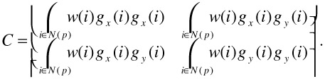

This increases the weight of central pixels and the feature point is moved to the position of maximum gradient variance. Without this weighting, the best position to place the feature point is not unique. The detector response is equal as long as the corner is completely contained in the neighborhood window. A sample result of automatic feature point detection is shown in Figure 23.5b.

3.3.2 Refinement to Sub-Pixel Accuracy

The corner detector described so far locates feature points only up to integer position accuracy. If the true feature point is located near the middle between pixels, jitter may occur. This can be reduced by estimating the sub-pixel position of the feature point.

The refinement is computed independently for the x and y coordinate. In the following, we concentrate on the x direction. The y direction is handled similarly. For each feature point, we match a parabola

v(∆x) = a (∆x)² + b ∆x + c

through the Harris response surface r(x, y), centered at the considered feature point. The fitted parabola is defined by the values of r at the feature point position and its two neighbors. By setting Δx = x - x_p , where x_p is the feature point position (cf. Figure 23.7), we get

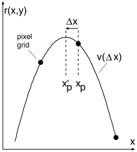
Figure 23.7: Sub-pel feature point localization by fitting a quadratic function through the feature point at x_p and its two neighbors.

(23.10)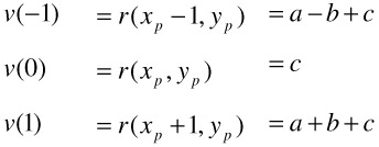

After setting dv / dΔx = 0, this leads to

(23.11)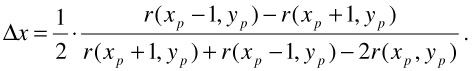

Since r(x_p, y_p) is a local maximum, it is guaranteed that | ∆x |<1. The new feature point position is set to the maximum of v, i.e., .

3.3.3 Determining Feature Correspondences

After appropriate feature points have been identified, we have to establish correspondences between feature points in successive frames. There are two main problems in establishing the correspondences. First, not every feature point has a corresponding feature point in the other frame. Because of image noise or object motion, new feature points may appear or disappear. Fortunately, the Harris corner detector is very stable so that most feature points in one frame will also appear in the next [19]. The second problem is that the matching can be ambiguous if there are several feature points surrounded by a comparable texture. This may happen, e.g., when there are objects with a regular texture or several identical objects in the image.

Let F₁, F₂ be the set of feature points of two successive images I₁,I₂. Our feature matching algorithm works as follows:

1. For each pair of features i ∈ F₁, j ∈ F₂ at positions (x_i; y_i), (x_j; y_j), calculate the matching error . f the Euclidean distance between the feature points exceeds a threshold td max, which is set to about 1/3 of the image width, d_i,j is set to infinity. The rationale for this threshold will be given shortly.

2. Sort all matching errors obtained in the last step in ascending order.

3. Discard all matches whose matching error exceeds a threshold t_{e max}.

4. Iterate through all pairs of feature points with increasing matching error. If neither of the two feature points has been assigned yet, establish a correspondence between the two.

Consequently, the matching process is a greedy algorithm, where best fits are assigned first. If there are single features without a counterpart, the probability that they will be assigned erroneously is low since all features that have correct correspondences have been assigned before and, thus, are not available for assignment any more. Moreover, the matching error will be high so that it will usually exceed t_d max.

There is one special case that justifies the introduction of te max. Consider a camera pan. Many feature points will disappear at one side of the image and new feature points will appear at the opposite side. After all feature points that appear in both frames are assigned, only those features at the image border remain. Thus, if the matching error is low, correspondences will be established between just to disappear and just appeared features across the complete image, which is obviously not correct. As we know that there will always be a large overlap between successive frames, we also know that the maximum motion cannot be faster than, say, 1/3 of the image width between frames. Hence, we can circumvent the problem by introducing the maximum distance limit t_{e max}.

3.3.4 Model Parameter Estimation by Least Squares Regression

Let , be the measured position of feature i, which had position x_i, y_i in the last frame. The best parameter set ? should minimize the squared Euclidean distance between the measured feature location and the position according to the camera model . Hence, we minimize the sum of errors

(23.12)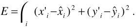

Using the affine motion model with θ = (a₁₁ a₁₂ t_x a₂₁ a₂₂ t_y ), we obtain the solution by setting the partial derivatives ∂E / ∂θ_i to zero, which leads to the following linear equation system:

(23.13)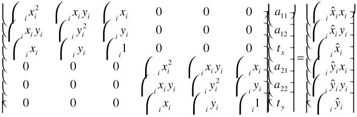

Clearly, this equation system can be solved efficiently by splitting it up into two independent 3 3 systems.

While this direct approach works for the affine motion model, it is not applicable to the perspective model because the perspective model is non-linear. One solution to this problem is that instead of using Euclidean distances

(23.14)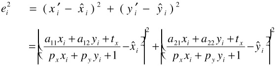

to use algebraic distance minimization, where we try to minimize the residuals

(23.15)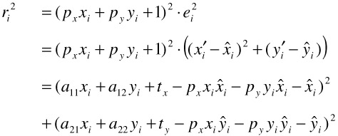

Note that because of the multiplication with (p_xx_i + p_yy_i + 1)², minimization of is biased, i.e., feature points with larger x_i, y_i have a greater influence on the estimation. This undesirable effect can be slightly reduced by shifting the origin of the coordinate system into the center of the image.

The sum of residuals can be minimized by a least squares (LS) solution of the overdetermined equation system

(23.16)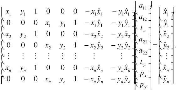

A number of efficient numerical algorithms (e.g., based on singular value decomposition) can be found for this standard problem in [15].

3.3.5 Robust Estimation

The main drawback of the LS method as described above is that outliers, i.e., observations that deviate strongly from the expected model, can totally offset the estimation result. Figure 23.8 illustrates this problem. For this purpose, we calculated motion estimates from two frames of a real-world sequence recorded by a panning camera. The motion vectors due to the pan are clearly visible in the background. In addition, the walking person in the foreground causes motion estimates that deviate from those induced by camera motion. Figure 23.8b displays the global motion field estimated by the LS method. Obviously, the mixture of background and object motion did not lead to satisfactory results. Instead, the camera parameters were optimized to approximate both, background and object motion.

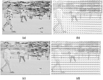
Figure 23.8: Estimation of camera parameters. (a) motion estimates, (b) estimation by least squares, (c) motion estimates (white vectors are excluded from the estimation), (d) estimation by least-trimmed squares regression.

In order to estimate camera parameters reliably from a mixture of background and object motion, one has to distinguish between observations belonging to the global motion model (inliers) and those resulting from object motion (outliers). Figure 23.8c displays the same motion estimates as before. This time, however, only a subset of vectors (drawn in black) is used for the LS estimation. The obtained camera motion model depicted in Figure 23.8d is estimated exclusively from inliers and, thus, clearly approximates the panning operation.

To eliminate outliers from the estimation process, one can apply robust regression methods. Widely used robust regression methods comprise random sample concensus (RANSAC) [4], least median of squares (LMedS), and least-trimmed squares (LTS) regression [17]. Those methods are able to calculate the parameters of our regression problem even when a large fraction of the data consists of outliers.

The basic steps are similar for all of those methods. First of all, a random subset of the data set is drawn and the model parameters are calculated from this subset. The subset size p equals the number of parameters to be estimated. For instance, calculating the 8 parameters of the perspective model requires 4 feature correspondences, each introducing two constraints. A randomly drawn subset containing outliers results in a poor parameter estimation. As a remedy, N subsets are drawn and the parameters are calculated for each of them. By choosing N sufficiently high, one can assure up to a certain probability that at least one "good" subset, i.e., a sample without outliers, was drawn. The probability for drawing at least one subset without outliers is given by P(ε, p, N) := 1 - (1 - (1 - ε)^p)^N where ε denotes the fraction of outliers. Conversely, the required number of samples to ensure a high confidence can be determined from this equation.

For each parameter set calculated from the subsets, the model error is measured. Finally, the model which fits the given observation best is retained. The main difference between the three methods RANSAC, LMedS, and LTS is the measure for the model error. We have chosen to use the LTS estimator because it does not require a selection threshold as RANSAC and it is computationally more efficient than LmedS [18]. The LTS estimator can be written as

(23.17)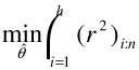

where n is the input data size and (r²)_1:n ≤?≤(r²)_n:n denote the squared residuals given in ascending order. Similar to the LS method, the sum of squared residuals is minimized. However, only the h smallest squared residuals are taken into account. Setting h approximately to n/2 eliminates half of the cases from the summation; thus, the method can cope with about 50% outliers.

Since the computation of the LTS regression coefficients is not straightforward, the basic steps are summarized in the following. For a detailed treatment and a fast implementation called FAST-LTS, we refer to [17,18].

To evaluate Equation 23.17, an initial estimate of the regression parameters is required. For this purpose, a subset S₀ of size p is drawn randomly from the data set. Solving a linear system created by S₀ yields an initial estimate of the parameters denoted by . Using we can calculate the residuals r_0i, i = 1,...,n for all n cases in the data set.

The estimation accuracy is increased by applying several compaction steps. Sorting r_0i by absolute value yields a subset H₀ containing the h cases with the least absolute residuals. Furthermore, a first quality of fit measure can be calculated from this subset as 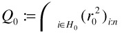. Then, based on H₀, a least squares fit is calculated yielding a new parameter estimate . Again, the residuals r_1i are calculated and sorted by absolute value in ascending order. This yields a subset H₁ which contains the h cases that possess the least absolute residuals with respect to the parameter set . The quality of fit for H₁ is given by 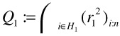. Due to the properties of LS regression, it can be assured that Q₁ ≤ Q₀. Thus, by iterating the above procedure until Q_k = Q_k-1, the optimal parameter set can be determined for a given initial subset.

3.4 Direct Methods for Motion Estimation

Although motion estimation based on feature correspondences is robust and can handle large motions, it is not accurate enough to achieve sub-pixel registration. Particularly in the process of building the background mosaic, small errors quickly sum up and result in clear misalignments. Given a good initial motion estimate from the feature matching approach, a very accurate registration can be calculated using direct methods. These techniques minimize the motion compensated image difference given as

(23.18)

I(x, y) denotes the image brightness at position (x, y) and I'(x',y') denotes the brightness at the corresponding pixel (according to the selected motion model) in the other image. For the moment, we assume that γ(e) = e², i.e., we use the sum of squared differences as difference measure. Later, we will replace this by a robust M-estimator.

Minimization of E with respect to the motion model parameter vector θ is a difficult problem and can only be tackled with gradient descent techniques. We are using a Levenberg-Marquardt [9, 11, 15] minimizer because of its stability and speed of convergence. The algorithm is a combination of a pure gradient descent and a multi-dimensional Newton algorithm.

3.4.1 Levenberg-Marquardt-Minimization

Starting with an estimation θ⁽ⁱ⁾, the gradient descent process determines the next estimation θ⁽ⁱ⁺¹⁾ by taking a small step down the gradient

(23.19)

where α is a small constant, determining the step size. One problem of pure gradient descent is the choice of a good α since small values result in a slow convergence rate, while large values may lead far away from the minimum.

The second method is the Newton algorithm. This algorithm assumes that if θ⁽ⁱ⁾ is near a minimum, the function to be minimized can often be approximated by a quadratic form Q as

(23.20)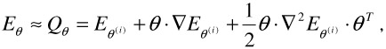

where ∇²E denotes the Hessian matrix of E.

If the Hessian matrix is positive definite,

(23.21)

Hence, because of

(23.22)

we can directly jump to the minimum of Q by setting

(23.23)

Note the similar structure of this equation compared to Equation 23.19. Instead of taking the inverse of the Hessian, the step δθ⁽ⁱ⁾ = θ⁽ⁱ⁺¹⁾ - θ⁽ⁱ⁾ can also be computed by solving the linear equation system

(23.24)

The Levenberg-Marquardt algorithm solves two problems at once. First, the factor a in Equation 23.19 is chosen automatically, and second, the algorithm combines steepest descent and Newton minimization into a unified framework.

If we are comparing the units of δθ⁽ⁱ⁾ with those in the Hessian, we can see that only the diagonal entries of the Hessian provide some information about scale. So, we set the step size (independently for each component θ_k) as

(23.25)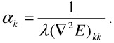

λ is a new scaling factor which is controlled by the algorithm. To combine steepest descent with the Newton algorithm, [9, 11] propose to define a new matrix D with

djk = (∇2E)jk	for j ≠ k
dkk = (∇2E)kk (l + λ)	(elements on the diagonal)

Replacing the Hessian of Equation 23.24 with D , we get

(23.26)

Note that for λ = 0 Equation 23.26 reduces to Equation 23.24 (i.e., the Newton algorithm), while for large λ the matrix D becomes diagonal dominant and the algorithm thus behaves like a steepest descent algorithm. The Levenberg-Marquardt minimization algorithm uses λ to control the minimization process and works as follows:

1. Choose an initial λ (e.g., λ = 0.001).

2. Solve Equation 23.26 to get the parameter update vector δθ⁽ⁱ⁾.

3. If ≥ , the update does not improve the solution. Hence, we increase λ by a factor of 10 (to reduce the step size) and go back to Step 2.

4. If < , the update improves the solution. Hence, we set θ⁽ⁱ⁺¹⁾ = θ⁽ⁱ⁾ + δθ⁽ⁱ⁾ and decrease λ by a factor of 10.

5. When λ exceeds a high threshold, even the last small steps did not improve the solution and we stop.

Adapting this technique to our motion estimation problem, we must determine the Hessian matrix and gradient vector for a given parameter estimate θ. In the following, we assume the perspective motion model from Equation 23.4. The gradient vector can be determined easily from

(23.27)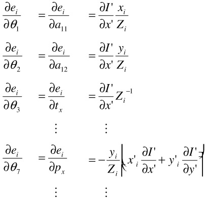

with the shortcut Z_i = p_xx_i + p_yy_i +1. Hence, with γ(e) = e² the gradient vector is simply

(23.28)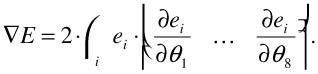

We simplify the computation of the Hessian by ignoring the second order derivative terms:

(23.29)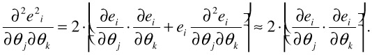

Hence, we get

(23.30)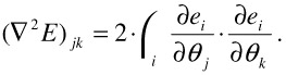

3.4.2 Applying an M-estimator

The algorithm described above assumes that the whole image moves according to the estimated motion model. However, in our application, this is not the case since foreground objects generally move differently. This introduces large matching errors in areas of the foreground objects. The consequence is that this mismatch distorts the estimation because the algorithm also tries to minimize the matching error in the foreground region. As the true object position is not known yet, it is not possible to exclude the foreground regions from the estimation process. This problem can be alleviated by using a limited error function for γ(x) instead of the squared error. For simplicity, we use

(23.31)

Introducing this error function into Equation 23.18 and computing the gradient and Hessian is particularly simple as

(23.32)

Figure 23.9 shows two difference frames, the first using squared error as matching function and the second using the robust distance function. It can be seen that the registration error in the background region is smaller for the robust distance function.

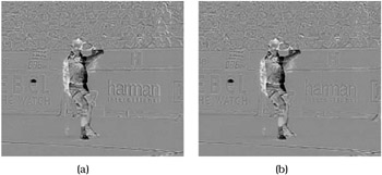
Figure 23.9: Difference frame after Levenberg-Marquardt minimization. (a) shows residuals using squared differences as error function, (b) shows residuals with saturated squared differences. It is visible that the robust estimation achieves a better compensation. Especially note the text in the right part of the image.