Changing the Appearance of Data | MicrosoftВ® Office ExcelВ® 2003 Step by Step (Step By Step (Microsoft))

Excel spreadsheets can hold and process lots of data, but when you manage numerous spreadsheets it can be hard to remember from a worksheet s title exactly what data is kept in that worksheet. Data labels give you and your colleagues information about data in a worksheet, but it s important to format the labels so that they stand out visually. To make your data labels or any other data stand out, you can change the format of the cells in which the data is stored.

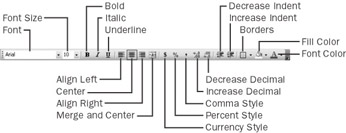
Most of the tools you need to change a cell s format can be found on the Formatting toolbar.

Important

Depending on the screen resolution you have set on your computer and which toolbar buttons you use most often, it s possible that not every button on every toolbar will appear on your Excel toolbars . If a button mentioned in this book doesn t appear on a toolbar, click the Toolbar Options button he small arrow at the right endof a toolbar to display the rest of its buttons.

You can apply the formatting represented by a toolbar button by selecting the cells you want to apply the style to and then clicking the appropriate button. If you want to set your data labels apart by making them appear bold, click the Bold button. If you have already made a cell s contents bold, selecting the cell and clicking the Bold button will remove the formatting.

Tip	Deleting a cell s contents doesn t delete the cell s formatting. To delete a cell s formatting, select the cell and then, on the Edit menu, point to Clear and click Formats.

Items on the Formatting toolbar that give you choices, such as the Font Color control, have a down arrow at the right edge of the control. Clicking the down arrow displays a list of options accessible for that control, such as the fonts available on your system or the colors you can assign to a cell.

Another way you can make a cell stand apart from its neighbors is to add a border around the cell. In versions of Excel prior to Excel 2002, you could select the cell or cells to which you wanted to add the border and use the options available underthe Formatting toolbar s Borders button to assign a border to the cells. For example, you could select a group of cells and then choose the border type you wanted. That method of adding borders is still available in Excel, but it has some limitations. The most important limitation is that, while creating a simple border around a group of cells is easy, creating complex borders makes you select different groups of cells and apply different types of borders to them. The current version of Excel makes creating complex borders easy by letting you draw borders directly on the worksheet.

To use the new border-drawing capabilities, display the Borders toolbar.

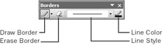
To draw a border around a group of cells, click the mouse pointer at one corner of the group and drag it to the diagonal corner. You will see your border expand as you move the mouse pointer. If you want to add a border in a vertical or horizontal line, drag the mouse pointer along the target grid line ”Excel will add the line without expanding it to include the surrounding cells. You can also change the characteristics of the border you draw by using the options on the Borders toolbar.

Another way you can make a group of cells stand apart from its neighbors is to change their shading, or the color that fills the cells. On a worksheet with monthly sales data for The Garden Company, for example, owner Catherine Turner could change the fill color of the cells holding her data labels to make the labels stand out even more than by changing the formatting of the text used to display the labels.

If you want to change the attributes of every cell in a row or column, you can click the header of the row or column you want to format and select your desired format.

One task you can t perform using the tools on the Formatting toolbar is to change the standard font for a workbook, which is used in the Name box and in the formula bar. The standard font when you install Excel is Arial, a simple font that is easy to readon a computer screen and on the printed page. If you want to choose another font, click Options on the Tools menu, which displays the General tab page, and use the Standard Font and Size controls to set the new default for your workbook.

Important

The new standard font won t take effect until you quit Excel and restart the program.

In this exercise, you emphasize a worksheet s title by changing the format of cell data, adding a border to a cell, and then changing a cell s fill color. After those tasks are complete, you change the default font for the workbook.

BE SURE TO start Excel before beginning this exercise.

USE the Formats.xls document in the practice file folder for this topic. This practice file is located in the My Documents\Microsoft Press\Office 2003 SBS\ChangingDocAppearance folder, and can also be accessed by clicking Start/All Programs/Microsoft Press/Microsoft Office System 2003 Step by Step .

OPEN the Formats.xls document.

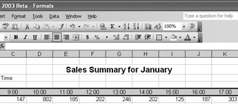
If necessary, click the January sheet tab.
Click cell E2.

Cell E2 is highlighted.
On the Formatting toolbar, click the Font Size down arrow and, from the list that appears, click 14 .

The text in cell E2 changes to 14-point type, and row 2 expands vertically to accommodate the text.
On the Formatting toolbar, click the Bold button.

The text in cell E2 appears bold.
Click the row head for row 5.

Row 5 is highlighted.
On the Formatting toolbar, click the Center button.

The contents of the cells in row 5 are centered.
Click cell E2.

Cell E2 is highlighted.
On the Formatting toolbar, click the down arrow at the right of the Borders button and then, from the list that appears, click Draw Borders .

The Borders toolbar appears, and the mouse pointer changes to a pencil.
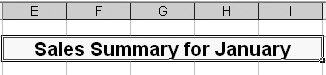
Click the left edge of cell E2 and drag to the right edge.

A border appears around cell E2.
On the Borders toolbar, click the Close button.

The Borders toolbar disappears.
On the Formatting toolbar, click the Fill Color down arrow.

The Fill Color color palette appears.
In the Fill Color color palette, click the yellow square.

Cell G2 fills with a yellow background.
On the Tools menu, click Options .

The Options dialog box appears.
If necessary, click the General tab. Click the Standard Font down arrow and select Courier New .
Click the Size down arrow, select 9 , and click OK .
Click OK to clear the dialog box that appears.
On the Standard toolbar, click the Save button.

Excel saves your changes.

CLOSE the Formats.xls document.