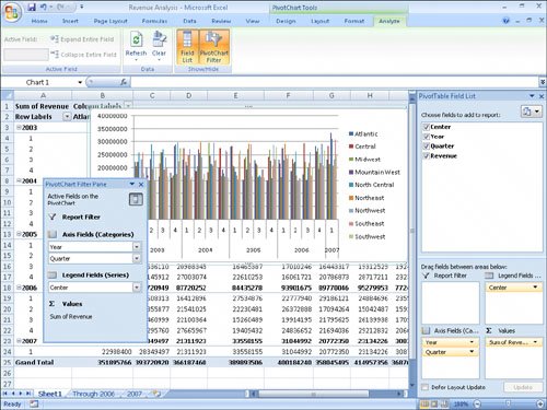
Creating Dynamic Charts Using PivotCharts

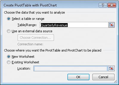
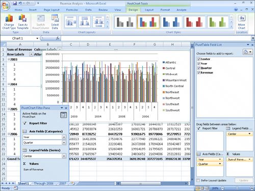
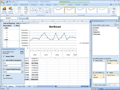
Just as you can create tables that you can reorganize on the fly to emphasize different aspects of the data in a list, you can also create dynamic charts, or PivotCharts, to reflect the contents and organization of a PivotTable.

Creating a PivotChart is fairly straightforward. Just click any cell in a list or data table you would use to create a PivotTable, and then click the Insert tab. In the Tables group, click the PivotTable button down arrow and then click PivotChart. In a worksheet with an existing PivotTable, click a cell in the PivotTable, display the Insert tab, and then, in the Charts group, click the type of chart you want to create.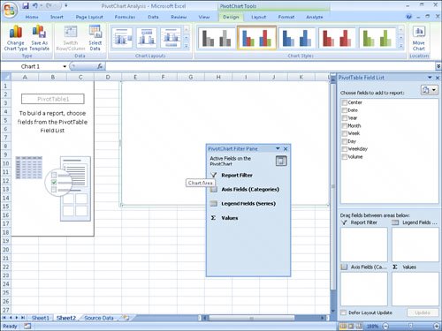

Any changes to the PivotTable on which the PivotChart is based are reflected in the PivotChart. For example, if the data in an underlying data list changes, clicking the Refresh Data button on the Options contextual tab, in the Data group, will change the PivotChart to reflect the new data. Also, you can filter the contents of the PivotTable shown here by clicking the Year down arrow, clicking 2003 from the list that appears, and then clicking OK. The PivotTable then shows revenues from 2003. The PivotChart also reflects the filter.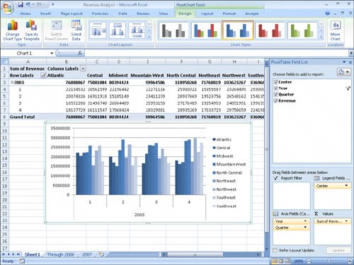

See Also

For more information on manipulating PivotTables, see "Creating Dynamic Lists with PivotTables" in Chapter 10.

The PivotChart has controls with which you can filter the data in the PivotChart and PivotTable. Clicking the Weekday down arrow, clicking (All) from the list that appears, and then clicking OK will restore the PivotChart to its original configuration.

If you ever want to change the chart type of an existing chart, you can do so by selecting the chart and then, on the Design tab, in the Type group, clicking Change Chart Type to display the Change Chart Type dialog box. When you select the desired type and click OK, Excel 2007 re-creates your chart.

Important

If your data is the wrong type to be represented by the chart type you select, Excel 2007 displays an error message.

In this exercise, you create a PivotTable and associated PivotChart, change the underlying data and update the PivotChart to reflect that change, and then change the PivotChart's type.

USE the Revenue Analysis workbook in the practice file folder for this topic. This practice file is located in the My Documents\Microsoft Press\Excel SBS\Charting folder.

OPEN the Revenue Analysis workbook.

1.	On the Through 2006 worksheet, click any cell in the data table.
2.	On the Insert tab, in the Tables group, click the PivotTable button down arrow and then click PivotChart. The Create PivotTable with PivotChart dialog box appears.
3.	Verify that the QuarterlyRevenue table appears in the Table/Range field and that the New Worksheet option button is selected.
4.	Click OK. Excel 2007 creates the PivotTable and associated PivotChart.
5.	In the PivotTable Field List task pane, drag the Center field header from the Choose fields to add to report area to the Legend Fields area.
6.	In the PivotTable Field List task pane, drag the Year field header from the Choose fields to add to report pane to the Axis Fields area.
7.	In the PivotTable Field List task pane, drag the Quarter field header from the Choose fields to add to report area to the Axis Fields area, positioning it below the Year field header.
8.	In the PivotTable Field List task pane, drag the Revenue field header from the Choose fields to add to report area to the Values area. Excel 2007 updates the PivotChart to reflect the field placements.
9.	On the tab bar, click the 2007 sheet tab. The 2007 worksheet appears.
10.	Select the data in cells B2:E10 and then press . Excel 2007 copies the data to the Clipboard.
11.	On the tab bar, click the Through 2006 sheet tab. The Through 2006 sheet tab appears.
12.	Select cell B147 and then press . Excel 2007 pastes the data into the worksheet and includes it in the table.
13.	On the tab bar, click the tab of the worksheet that contains the PivotChart. The PivotChart appears.
14.	Select the PivotChart and then, on the Analyze contextual tab, in the Data group, click Refresh. Excel 2007 adds the new table data to your PivotChart.
15.	On the Design contextual tab, in the Type group, click Change Chart Type. The Change Chart Type dialog box appears.
16.	Click Line and then click the second Line chart subtype.
17.	Click OK. Excel 2007 changes your PivotChart to a line chart.
18.	In the PivotTable Field List, in the Choose fields to add to report area, click the Center field header.
19.	Click the down arrow that appears and then, in the menu that appears, clear the Select All check box. Excel 2007 removes the check boxes from the filter list items.
20.	Select the Northeast check box and then click OK. Excel 2007 filters the PivotChart.

CLOSE the Revenue Analysis workbook.