12.3 Case II: Multiple server computer system

---

12.3 Case II: Multiple server computer system

Another classic analysis is that of the multiprocessor. In this case, we can replace the central server model with multiple examples of the same model cascaded together (Figure 12.4), or we could examine more elaborate implementations-for example, the shared memory model (Figure 12.5a) or the multiple bank shared memory model (Figure 12.5b).

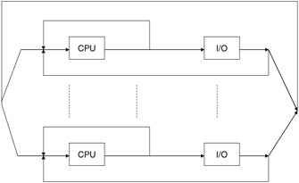
Figure 12.4: Multiprocessor model using central processor.

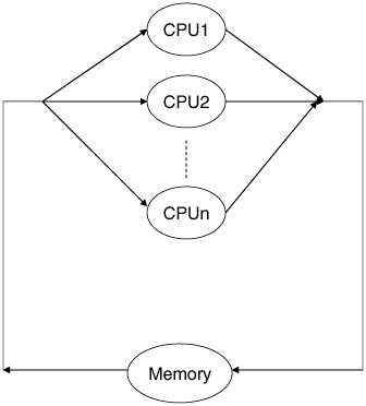
Figure 12.5a: Shared memory model.

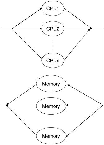
Figure 12.5b: Multibank shared memory model.

The analysis of any one of these architectures would follow methodology similar to that of the single CPU case described previously. The system we choose to model here is the multiprocessor case. This is more indicative of realistic systems, where multiple servers are interconnected to serve several users.

If we decide to model the system shown in Figure 12.5b, we have essentially the problem of memory allocation to processors. A processor can have all of the memory or none of the memory or anything in between. Allocations are done using the entire memory module. That is, a CPU cannot share a memory module with another CPU during a cycle.

On each CPU cycle, each processor makes a memory request. If there is a free memory meeting the CPU's request, it gets filled; otherwise, the CPU must wait until the next cycle. Each memory module for which there is a memory access request can fill only one request. When several processors make memory module requests to the same memory module, only one is served (chosen at random from those requesting). The other processors will make the same memory module request on the next cycle. New memory requests for each processor are chosen randomly from the M memory modules using a uniform distribution.

Let the system state be the number of memory requests for each memory module:

(12.6) 

where k_i represents the memory request by processors for memory bank i.

At the start of a cycle the sum of all requests cannot exceed the number of processors in the system, N:

(12.7) 

The total number of possible states is related to the number of ways N processor requests can be distributed to M memory modules:

(12.8)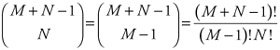 

or, in other terms, how to allocate N balls to M cells.

For N = 2 and M = 4 (see Figure 12.6) the possible way to allocate the four memory modules to processors (indistinguishable from each other) is shown in Table 12.1.

Table 12.1: Possible Ways to Allocate Memory

Memory
	1	2	3	4
1	0	0	0	2
2	0	0	1	1
3	0	0	2	0
4	0	1	0	1
5	0	1	1	0
6	0	2	0	0
7	1	0	0	1
8	1	0	1	0
9	1	1	0	0
10	2	0	0	0

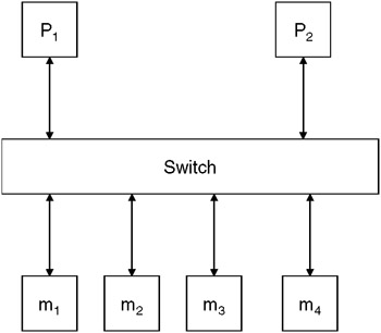
Figure 12.6: Multiprocessor system with N = 2 and M = 4.

and is found by:

(12.9) 

We can see that if the number of processors requesting memory modules and the number of memory modules are increased, the number of possible states grows very quickly, making this analysis difficult for even relatively small problems, as shown in Table 12.2.

Table 12.2: Number of States for Selected Number of Processors and Memory Modules

N	M	# States
2	4	10
3	5	35
4	7	210

Let H = (h₁,h₂,...,h_m) represent the intermediate state, when the memory access requested on a cycle has been filled and the new requests have not yet been made:

(12.10) 

Let G represent a new (feasible) system state:

(12.11) 

First, let's define:

(12.12) 

Note 

The state G can be reached from state K in one cycle if, and only if, d_i ≥ 0 for each i.

12.3.1 Properties

1. If G is reachable from K in one cycle, the probability it will in fact be the next state is given by:

   (12.13) 

   

   where x represents the number of new requests.

2. The system can be described by a Markov chain, since the next state probabilities at any time depend only on the current state.

3. The system is aperiodic, since a one-step transition from a state to itself is possible at any time.

4. The system is irreducible, since it can reach any other in a finite number of steps.

Hence, since it is a finite state process, it is also an ergotic Markov process. Also, since these conditions hold, there is an equilibrium state probability distribution, Π, so that:

(12.14) 

where P is the state transition matrix (described in Chapters 6 and 7):

(12.15) 

A performance assessment typically made in such system configurations to determine what the effective processor power of the N processors with M memory system is:

(12.16) 

Let Proc(i) represent the number of memory requests serviced (instructions executed) when the system is in state i:

(12.17) 

For the simple case where N = 2 and M = 2, we have the system illustrated in Figure 12.7.

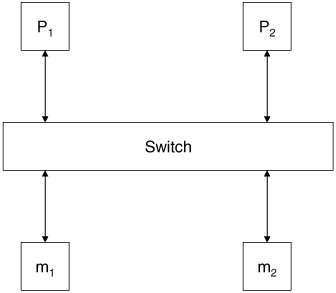
Figure 12.7: Multiprocessor system with N = 2 and M = 2.

The possible states this model could be in, representing the requested memory requested by the two processors, is described as (see Figure 12.8):

(12.18)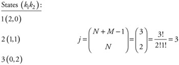 

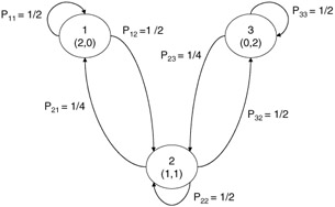
Figure 12.8: Probability state transition diagram.

Using the general formula:

(12.19)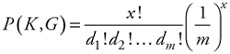 

(12.20) 

which represents the probability of being in state (2,0) and transitioning to state (1,1). Similarly, the probability of being in state (1,1) and traversing to state (2,0) would be found as:

(12.21)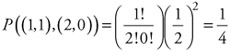 

and so on.

The balance equations for this Markov chain can be found using the relationship:

(12.22) 

(12.23) 

Solving these simultaneous equations yields:

(12.24)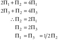 

and since:

(12.25) 

then:

(12.26) 

The discovered effective processor power is computed using the relationship:

(12.27) 

where

i	Proc(i) number of instructions executed in state i:
1	1
2	2
3	1

(12.28) 

Results for M memory modules (2 ≤ M ≤ 10) and N processors (2 ≤ N ≤ 5) are summarized in Table 12.3.

Table 12.3: Summary of Speed Up for M Memory and N Processors

M	N Processors
Memory Modules	2	3	4	5
2	1.5	-	-	-
3	1.667	2.048	-	-
4	1.750	2.269	2.62	-
5	1.800	2.409	2.863	3.199
6	1.833	2.505	3.036	3.453
7	1.857	2.575	3.166	3.648
8	1.875	2.627	3.265	3.801
9	1.889	2.668	3.344	3.925
10	1.900	2.701	3.407	4.025

Limitations: The model does not take into account memory interference caused by I/O operations. It also assumes the processors and memory are synchronized, as are memory access/cycle.

---