12.2 Case 1: Central server computer system

---

12.2 Case 1: Central server computer system

The central server model, shown in Figure 12.1, is typical of most desktop computers and single processor servers in service today. The main elements of this model are the CPU, memory, and I/O devices (disks, network connections, etc.). In addition to these major components, the model must also depict how these components are connected to each other, forming the architecture of the central server computer system. The interconnection would consist of paths for new program initiation and for active programs to circulate through the system. The assumption here is that the number of jobs (programs) circulating in the system is steady and fixed. Each of the fixed number of jobs performs some CPU activity, followed by some I/O activity, and back to the CPU for additional service.

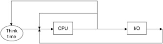
Figure 12.1: Central server model.

The modeled system would be typical of computers one would find on a person's desk in a high-capacity business office. Such a computer system would consist of a single CPU (such as a Pentium IV with onboard cache), matched speed main memory (128 MB to 1 GB), at least one disk drive, and numerous other peripheral devices. The machine would also be connected to the Internet and may service remote service calls. The operating system is one of the industry standards (Microsoft XP, LINUX).

The processing capacity of the CPU and each of the I/O devices is denoted by μ_i = 1/T_S(i), where T_S(i) is the average service time for the specified device. The flow of control for a job in the system is directed by the branching probabilities, p₁,p₂,p₃,...,p_n. On leaving the CPU a job may loop back to the CPU for more service, with probability p₁. The interpretation of this can be that the program is going back for more service, or it is completing and being replaced by another new program.

The remaining values are easier to interpret. The probabilities p₂,p₃,...,p_n determine what percentage of I/O requests go to which device. From earlier chapters you will recall that:

(12.1)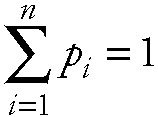 

The value μ_i, i = 1,2,...,n, represents the service rates for each defined server in the model. The service rate is the number of instructions performed divided by the raw speed of the device. For example, the CPU service rate is defined as:

(12.2) 

In most analyses we make the assumption that the service discipline is FCFS and that the arrival rate and service rates are exponentially distributed and the queuing discipline is FCFS. The key metrics we are interested in discovering are throughput and utilization.

The typical method to compute this is to use Buzen's algorithm. This algorithm determines the probability of having different numbers of jobs in different servers at a point in time. The number of jobs at any particular node is not independent of the remainder of the systems nodes, since the total number in the system must be kept steady. This algorithm proves that the probability of the jobs being spread around the servers in a particular distribution is:

(12.3) 

Using this property and Little's Law we can compute some of the metrics of interest as:

(12.4)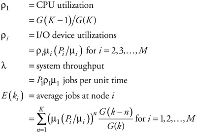 

One of the most important components of Buzen's algorithm is the function G(k) for k = l,2,3,...,M. To perform this computation a partial function g(k,m) is defined. The details of this function were provided in Chapter 7. Repeating some of the important aspects of computing G(k):

(12.5)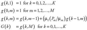 

Details of the solution can be found in [9].

As an example of the operation of this algorithm we can set some of the values for a test system. If we assume we have a system with a CPU and three I/O devices, M = 4. We can set the service rate for the I/O devices as all the same μ₂ = μ₃ = μ₄ = 10 I/Os per second. The CPU is set at μ₁ = 18.33 quantum slices per job. If we set K = 8 tasks circulating through the system and run it through Buzen's algorithm we would find the results shown in the following chart.

CPU Time per Request	Disk I/O Rate	CPU Utilization	Disk Utilization	Throughput Requests/sec
0.6	10	0.96	0.53	1.6
0.3	10	0.67	0.74	2.23
0.6	15	1.00	0.37	1.66
0.3	15	0.88	0.65	2.92

A similar analysis could be developed using a Petri net instead of the queuing model. Figure 12.2 depicts a Petri net example for the single I/O device system shown in Figure 12.1.

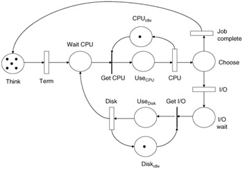
Figure 12.2: Central server Petri net.

In the depicted model, jobs get submitted through a set of terminals represented by the think place and the term transition. Once a job is requesting service, it is moved into the wait CPU place to wait for the CPU to become available. Once it is available, the waiting job acquires the CPU and models using it by moving into the use CPU place, followed by the CPU transition, which models the execution cycle of the CPU. After a job has completed its use of the CPU, it moves to the choose place. In this place a decision must be made to check if the job is complete or if more I/O is needed. If completed, the token representing a job moves back to the think place to become a new job later. If I/O is needed, the token moves to the disk wait place to busy wait for the disk resource. Once the resource is freed, the job acquires the disk and models using the disk by moving into the use disk place followed by enabling of the disk transition. Upon completion of disk use, the token (job) goes back into the wait CPU place to reacquire the CPU. If we wish to model more disk drives, we simply make more branches from the choose place and replicate the loop for the disk drive (Figure 12.3).

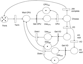
Figure 12.3: Multiple disk example Petri net.

If we set the timed transitions as follows: Term 0.1, CPU 1.0, and Disk at 0.8, and the places initially loaded with tokens as: think = 6, CPU_idle = 1, and Disk_idle = 1, we can proceed with the analysis. The first analysis must be to determine if the model is bounded and live. That is to say, there are no deadlock states and the net is configured so it can initiate firings. By examining this net we can also see that there are four major place flows through the net. Flow 1 = think, wait CPU, Use CPU, and Choose. Flow 2 = If we set = think, wait CPU, Use CPU, Choose, diskwait, and use disk. Flow 3 = CPUidle, useCPU. Flow 4 = diskidle, use disk. The first flow corresponds to jobs using the CPU and completing with no need for I/O. The second flow also represents jobs using the CPU but also requiring and using I/O devices. The third flow loop represents the CPU cycle of busy and idle, and the final flow loop represents the disk cycle of busy and idle time. Since all of the places of the Petri net are covered by these flows, the net is bounded. This also implies that this network has a finite reachability graph, and, therefore, the underlying Markov chain has a finite state space.

Using these flows we can compute the average time for jobs to flow through each loop by running this model. If we ran the model with the same data as in the queuing model, the same results would follow. More details about this model and others can be found in [10].

---