8.3 Systems and modeling

---

8.3 Systems and modeling

Up to this point, we have discussed generic attributes related to simulation modeling. We have not discussed the classes of modeling techniques available or the classification of simulation implementation techniques (i.e., simulation languages). Simulation techniques include discrete event, continuous change, queuing, combined, and hybrid techniques. Each provides a specific viewpoint to be applied to the simulation problem. They will also force the modeler to fit models to the idiosyncrasies of the techniques.

8.3.1 Discrete models

In discrete simulation models, the real system's objects are typically referred to as entities. Entities carry with them attributes that describe them (i.e., their state description). Actions on these entities occur on boundary points or conditions. These conditions are referred to as events. Events such as arrivals, service standpoints, stop points, other event signaling, wait times, and so on are typical.

The entities carry attributes that provide information on what to do with them based on other occurring events and conditions. Only on these event boundaries or condition occurrences can the state of entities change. For example, in our bank teller simulation, only on an arrival of a customer (arrival event) can a service event be scheduled, or only on a service event can an end of service event be scheduled. This implies that without events the simulation does not do anything. This modeling technique only works on the concept of scheduling events and acting on them. Therefore, it is essential that the capability exists to place events into a schedule queue or list and to remove them based on some conditions of interest.

What this technique implies is that all actions within the simulation are driven by the event boundaries. That is, event beginnings and endings can be other events to be simulated (i.e., to be brought into action). All things in between these event boundaries, or data collection points, are now changing. A simulation model using this technique requires the modeler to define all possible events within the real system and how these events affect the state of all the other events in the system. This process includes defining the events and developing definitions of change to other states at all event boundaries, of all activities that the entities can perform, and of the interaction among all the entities within the simulated system. In this type of simulation modeling each event must trigger some other event within the system. If this condition does not hold, we cannot construct a realistic working simulation. This triggering provides the event's interaction and relationship with each other event. For example, for the model of a self-service automatic teller machine, we need to define at a minimum the following entities and events:

• Arrival events

• Service events

• Departure events

• Collection events

• Customer entities

• Server entities

The events guide how the process occurs and entities provide the medium being acted on, all of which are overseen by the collection event that provides the "snapshot" view of the system. This provides a means to extract statistics from entities. In this example, the following descriptions could be used to build a simple model:

1. Arrival event

   • Schedule next arrival (present time + T).

   • If all tellers busy, number waiting = number waiting + 1.

   • If any teller is free and no one is before the waiting customer, schedule service event.

2. Service event

   • Number of tellers busy = number of tellers busy + 1.

   • Schedule service and event based on type of service.

   • Take start of service statistics.

3. End service event

   • Number of tellers busy = number tellers busy - 1.

   • Schedule arrival of customer.

   • Take end of service statistics.

4. Entities

   • Tellers

     • Number of tellers

     • Service rates and types

     • Service types

   • Customers

     • Arrival rate

     • Dynamics (service type required)

A discrete event simulation (with an appropriate language) could be built using these events and entities as their basis. A model built this way uses these conditions to schedule some number of arrivals and some end conditions. The relationships that exist between the entities will keep the model executing, with statistics taken until the end condition is met. This example is extremely simplistic and by no means complete, but it does provide a description of some of the basic concepts associated with discrete event simulations.

8.3.2 Continuous modeling

Continuous simulations deal with the modeling of physical events (processes, behaviors, conditions) that can be described by some set of continuously changing dependent variables. These in turn are incorporated into differential, or difference, equations that describe the physical process. For example, we may wish to determine the rate of change of speed of a falling object shot from a catapult (see Figure 8.1) and its distance, R, from the catapault. Neglecting wind resistance, the equations for this are as follows. The velocity, v, at any time is found as:

(8.1)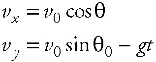 

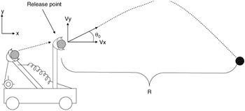
Figure 8.1: Projectile motion.

and the distance in the x direction is:

(8.2) 

These quantities can be formulated into equations that can be modeled in a continuous language to determine their state at any period of time t.

Using these state equations, we can build state-based changed simulations that provide us with the means to trigger on certain occurrences. For example, in these equations we may wish to trigger an event (shoot back when v_y is equal to 0). That is, when the projectile is not climbing any more and it has reached its maximum height, fire back. In this event the equation may look like this:

(8.3) 

Another example of this type of triggering is shown in Figure 8.2. In this example, two continuous formulas are being computed over time; when their results are equivalent (crossover event), schedule some other event to occur. This type of operation allows us to trigger new computations or adjust values of present ones based on the relationship of continuous equations with each other.

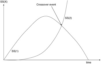
Figure 8.2: Continuous variable plot.

Using combinations of self-triggers and comparative triggers (less than, greater than, equal to, etc.) we can construct ever more involved simulations of complex systems. The main job of a simulator in this type of simulation model is to develop a set of equations that define the dynamics of the system under study and determine how they are to interact.

8.3.3 Queuing modeling

Another class of generic model is the queuing model. Queuing-based simulation languages exist (AWESIM, GPSS, Q-gert, Slam II) and have been used to solve a variety of problems. As was indicated earlier, many problems to be modeled can easily be described as an interconnection of queues, with various queuing disciplines and service rates. As such, a simulation language that supports queuing models and analysis of them would greatly simplify the modeling problem. In such languages there are facilities to support the definition of queues in terms of size of queue, number of servers, type of queue, queue discipline, server type, server discipline, creation of customers, monitoring of operations, departure collection point, statistics collection and correlation, and presentation of operations. In addition to basic services there may be others for slowing up customers or routing them to various places in the queuing network. Details of such a modeling tool will be highlighted later in this chapter.

8.3.4 Combined modeling

Each of the techniques described previously provides the modeler with a particular view upon which to fit the system's model. The discrete event-driven models provide us with a view in which systems are composed of entities and events that occur to change the state of these entities. Continuous models provide a means to perform simulations based on differential equations or difference formulas that describe time-varying dynamics of a system's operation. Queuing modeling provides the modeler with a view of systems comprised of queues and services. The structure comes from how they are interconnected and how these interconnections are driven by the outputs of the queue servers.

The problem with all three techniques is that in order to use them, a modeler must formulate the problem in terms of the available structure of the technique. It cannot be formulated in a natural way and then translated easily. The burden of fitting it into a framework falls on the modeler and the simulation language. The solution is to provide a combined language that has the features of all three techniques. In such a language the modeler can build simulations in a top-down fashion, leaving details to lower levels. For instance, in our bank teller system, we could initially model it as a single queue with n servers (tellers). The queuing discipline is first-come, first-served, and the service discipline can be any simple distribution, such as exponential. This simple model will provide us with a sanity check of the correctness of our model and with bounds to quickly determine the system's limits. We could next decide to model the teller's service in greater detail by dropping this component's level down to the event modeling level.

At this point we could model the teller's activity as a collection of events that need to be sequenced through in order for service to be completed. If possible, we could then incorporate continuous model aspects to get further refinement of some other feature. The main aspect to gather from this form of modeling is that it provides the modeler with the ability to easily model the level of detail necessary to simulate the system under study.

8.3.5 Hybrid modeling

Hybrid modeling refers to simulation modeling in which we incorporate features of the previous techniques with conventional programming languages. This form of modeling could be as simple as doing the whole thing in a regular language and allowing lower levels of modeling by providing a conventional language interface. Most simulation languages provide a means to insert regular programming language code into them. Therefore, they all could be considered a variant of this technique.

---