1.7 Overview of performance evaluation methods

< Free Open Study >

Models provide a tool for users to define a system and its problems in a concise fashion; they provide vehicles to ascertain critical elements, components, and issues; they provide a means to assess designs or to synthesize and evaluate proposed solutions; and they can be used as predictions to forecast and aid in planning future enhancements or developments. In short, they provide a laboratory environment in which to study a system even before it exists or without actually effecting an actual implementation. In this light models are descriptions of systems. Models typically are developed based on theoretical laws and principles. They may be physical models (scaled replicas), mathematical equations and relations (abstractions), or graphical representations. Models are only as good as the information put into them. That is, modeling of a system is easier and typically better if:

Physical laws are available that can be used to describe it.
Pictorial (graphical) representations can be made to provide better understanding of the model.
The system's inputs, elements, and outputs are of manageable magnitude.

These all provide a means to construct and realize models, but the problem typically is that we do not have clear physical laws to go by; interactions can be very difficult to describe; randomness of the system, environment, or users causes problems; and policies that drive processes are hard to quantify. What typically transpires is that a "faithful" model of a system is constructed: one that provides insight into a critical aspect of a system, not all of its components. That is, we typically model a slice of the real-world system. What this implies is that the model is an abstraction of the real-world system under study. With all abstractions, one must decide what elements of the real world to include in the abstraction-that is, which ones are important to realize as a "faithful" model. What we are talking about here is intuition-that is, how well a modeler can select the significant elements; how well these elements can be defined; and how well the interaction of these significant elements is within themselves, among themselves, and with the outside world.

1.7.1 Models

As stated previously, a model is an abstraction of a system. (See Figure 1.11.) The realism of the model is based on the level of abstraction applied. That is, if we know all there is about a system and are willing to pay for the complexity of building a true model, the abstraction is near nil. On the other hand, in most cases we wish to abstract the view we take of a system to simplify the complexities. We wish to build a model that focuses on some element(s) of interest and leave the rest of the system as only an interface with no detail beyond proper inputs and outputs.

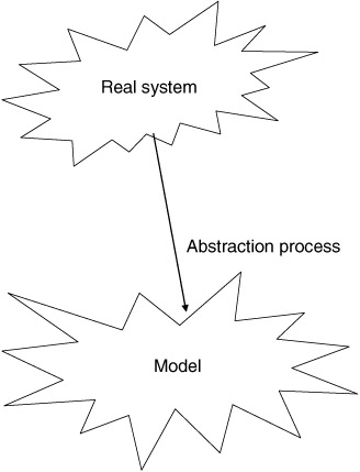
Figure 1.11: Modeling process.

The "system," as we have been calling it, is the real world that we wish to model (e.g., a bank teller machine, a car wash, or some other tangible item or process). In Figure 1.12 a system is considered to be a unified group of objects united to perform some set function or process, whereas a model is an abstraction of the system that extracts the important items and their interactions.

click to expand
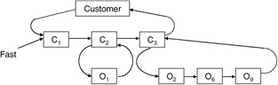
Figure 1.12: Abstraction of a system.

The basic concept of this discussion is that a model is a modeler's subjective view of the system. This view defines what is important, what the purpose is, detail, boundaries, and so on. The modeler must understand the system in order to provide a faithful perspective of its important features and to make the model useful.

1.7.2 Model construction

In order to construct a model, we as modelers must follow predictable methodologies in order to derive correct representations. The methodology typically used consists of top-down decomposition and is pertinent to the goal of being able to define the purpose of the model or its component at each step and, based on this purpose, to derive the boundaries of the system or component and develop the level of modeling detail. This iterative method of developing purpose, boundaries, and modeling level smooths out the rough or undefinable edges of the actual system or component, thereby focusing on the critical elements of it.

The model's inputs are derived from the system under study as well as from the performance measures we wish to extract. That is, the type of inputs are detailed not only from the physical system but through the model's intended use (this provides the experimental nature of the model). For instance, in an automated teller machine, we wish to study the usefulness of fast service features, such as providing cash or set amounts of funds quickly after the amount has been typed in. We may decide to ignore details of the ATM's internal operations or user changes.

The model would be the bank teller machine, its interface, and a model (analytical, simulation) of the internal process. The experiment would be to have users (experimenters) use the model as they would a real system and measure its effectiveness. The measures would deal with the intent of the design. That is, we would monitor which type of cash access feature was used over another, which performed at a higher level, or which features were not highly utilized.

The definition of the required performance measures drive the design and/or redesign of the model. In reality, the entire process of formulating and building a model of a real system occurs interactively. As insight is gained about the real system through studying it for modeling purposes, new design approaches and better models and components are derived. This process of iteration continues until the modeler has achieved a level of detail consistent with the view of the real system intended in the model-purpose development phase. The level of detail indicates the importance of each component in the modeler's eye as points that are to be evaluated.

To reiterate, the methodology for developing and using a model of a system is as follows:

Define the problem to be studied as well as the criteria for analysis.
Define and/or refine the model of the system (includes development of abstractions of the system into mathematical, logical, and procedural relationships).
Collect data for input to the model (define the outside would and what must be fed to or taken from the model to "simulate" that world).
Select a modeling tool and prepare and augment the model for tool implementation.
Verify that the tool implementation is an accurate reflection of the model.
Validate that the tool implementation provides the desired accuracy or correspondence with the real-world system being modeled.
Experiment with the model to obtain performance measures.
Analyze the tool results.
Use these findings to derive designs and improvements for the real-world system.

Although some of these steps were defined previously, they will be read-dressed here in the context of the methodology.

The first task in the methodology is to determine what the scope of the problem is and if this real-world system is amenable to modeling. This task consists of clearly defining the problem and explicitly delineating the objectives of the investigation. This task may need to be reevaluated during the entire model construction phase because of the nature of modeling. That is, as more insight comes into the process, a better model, albeit a different one, may be developed. This involves a redefinition of questions and the evolution of a new problem definition.

Once a problem definition has been formulated, the task of defining and refining a model of this real-world problem space can ensue. The model typically is made up of multiple sections that are both static and dynamic. They define elements of the system (static), their characteristics, and the ways in which these elements interact over time to adjust or reflect the state of the real system over time. As indicated earlier, this process of formulating a model is largely dependent on the modeler's knowledge, understanding, and expertise (art versus science). The modeler extracts the essence of the real-world system without encasing superfluous detail. This concept involves capturing the crucial (most important) aspects of the system without undue complexity but with enough to realistically reflect the germane aspects of the real system. The amount of detail to include in a model is based mainly on its purpose. For example, if we wish to study the user transaction ratio and types on an automated teller machine, we only need model the machine as a consumer of all transaction times and their types. We need not model the machine and its interactions with a parent database in any detail but only from a gross exterior user level.

The process of developing the model from the problem statement is iterative and time consuming. However, a fallout of this phase is the definition of input data requirements. Added work typically will be required to gather the defined data values to drive the model. Many times in model development data inputs must be hypothesized or be based on preliminary analysis, or the data may not require exact values for good modeling. The sensitivity of the model is turned into some executable or analytical form and the data can be analyzed as to their effects.

Once the planning and development of a model and data inputs have been performed, the next task is to turn it into an analytical or executable form. The modeling tool selected drives much of the remainder of the work. Available tools include simulation, analytical modeling, testbeds, and operational analysis. Each of these modeling tools has its pros and cons. Simulation allows for a wide range of examinations based on the modeler's expertise; analytical analysis provides best, worst, and average analysis but only to the extent of the modeler's ability to define the system under study mathematically. Testbeds provide a means to test the model on real hardware components of a system, but they are very expensive and cumbersome. Operational analysis requires that we have the real system available and that we can get it to perform the desired study. This is not always an available alternative in complex systems. In any case, the tool selected will determine how the modeler develops the model, its inputs, and its experimental payoff.

Once a model and a modeling tool to implement it have been developed, the modeler develops the executable model. Once developed, this model must be verified to determine if it accurately reflects the intended real-world system under study. Verification typically is done by manually checking that the model's computational results match those of the implementation. That is, do the abstract model and implemented model do the same thing and provide consistent results?

Akin to verification is validation. Validation deals with determining if the model's implementation provides an accurate depiction of the real-world system being modeled. Testing for accuracy typically consists of a comparison of the model and system structures against each other and a comparison of model tool inputs, outputs, and processes versus the real system for some known boundaries. If they meet some experimental or modeling variance criteria, we deem the model an accurate representation of the system. If not, the deficiencies must be found, corrected, and the model revalidated until concurrence is achieved.

Once the tool implementation of the model has been verified and validated, the modelers can perform the project's intended experiments. This phase is the one in which the model's original limitations can be stretched and new insights into the real system's intricacies can be gained. The limitations on experimentation are directly related to the tool chosen: Simulation is most flexible followed by testbeds, analytical analysis, and operational analysis.

Once experimentation is complete, an ongoing analysis of results is actively performed. This phase deals with collecting and analyzing experimentally generated data to gain further insight into the system under study. Based on the results generated, the modeler feeds these results into the decision-making process for the real-world system, potentially changing its structure and operations based on the model's findings. A study is deemed successful when the modeling effort provides some useful data to drive the end product. The outputs can solidify a concept about the system, define a deficiency, provide insight into improvements, or corroborate other information about the system. Modeling is a useful tool with which to analyze complex environments.

1.7.3 Modeling tools

As was briefly indicated in the previous section, there are major classes of modeling tools in use today: analytical, simulation, testbed, and operational analysis. Each has its niche in the modeler's repertoire of tools and is used for varying reasons, as will be discussed later in the book.

Analytical modeling tools

Analytical modeling tools have been used as an implementation technique for models for quite some time, the main reason being that they work. Analytical implementations of models rely on the ability of the modeler to describe a model in mathematical terms. Typically, if a system can be viewed as a collection of queues with service, wait, and analytical times defined analytically, queuing analysis can be applied to solve the problem. Other analytical tools such as Petri nets can also be applied to the solution of such problems.

Some of the reasons why analytical models are chosen as a modeling tool are as follows:

Analytical models capture more salient features of systems-that is, most systems can be represented as queuing delays, service times, arrival times, and so on, and, therefore, we can model from this perspective, leaving out details.
Assumptions or analysis is realistic.
Algorithms to solve queuing equations are available in machine form to speed analysis.

What is implied by this is that queuing models provide an easy and concise means to develop analysis of queue-based systems. Queues are waiting lines, and queuing theory is the study of waiting line dynamics.

In queuing analysis at the simplest level (one queue), there is a queue (waiting line) that is being fed by incoming customers (arrival rate); the queue is operated by a server, which extracts customers out of the queue according to some service rate (see Figure 1.13).

click to expand
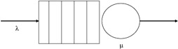
Figure 1.13: Single server queue.

The queue operates as follows: An arrival comes into the queue, and, if the server is busy, the customer is put in a waiting facility (the queue) unless the queue is full, in which case the customer is rejected (no room to wait). On the other hand, if the queue is empty, the customer is brought into the service location and is delayed the service rate time. The customer then departs the queue.

In order to analyze this phenomenon we need to have notational and analytical means (theories) with which to manipulate the notation. Additionally, to determine the usefulness of the technique, we need to know what can be analyzed and what type of measure is derived from the queue.

The notation used (see Figure 1.13) to describe the queue phenomenon is as follows: The arrival distribution defines the arrival patterns of customers into the queue. These are defined by a random variable that defines the interarrival time. A typically used measure is the Poisson arrival process, defined as:

(1.1)

where the average arrival rate is λ. The queue is defined as a storage reservoir for customers. Additionally, the policy it uses for accepting and removing customers is also defined. Examples of queuing disciplines typically used are first-in first-out (FIFO) and last-in first-out (LIFO). The last main component of the queue description is the service policy, which is the method by which customers are accepted for service and the length of the service. This service time is described by a distribution, a random variable. A typical service time distribution is the random service given by:

(1.2)

where t >> 0, and the symbol μ is reserved to describe this common distribution for its average service rate. The distributions used to describe the arrival rate and service ratios are many and variable; for example, the exponential, general, Erlang, deterministic, or hyperexponential can be used. The Kendall notation was developed to describe what type of queue is being examined. The form of this notation is as follows:

(1.3)

where A specifies the interarrival time distribution, B the service time distribution, c the number of servers, K the system capacity, m the number in the source, and Z the queue discipline.

This type of analysis can be used to generate statistics on average wait time, average length of the queue, average service time, traffic intensity, server utilization, mean time in system, and various probability of wait times and expected service and wait times. More details on this modeling and analysis technique will be presented in Chapter 7.

Simulation modeling tools

Simulation as a modeler's tool has been used for a long time and has been applied to the modeling and analysis of many systems-for example, business, economics, marketing, education, politics, social sciences, behavioral sciences, international relations, transportation, law enforcement, urban studies, global systems, computers, factories, and many more. Simulation lends itself to such a variety of problems because of its flexibility. It is a dynamic tool that provides the modeler with the ability to define models of systems and put them into action. It provides a laboratory in which to study myriad issues associated with a system without disturbing the actual system. A wide range of experiments can be performed in a very controlled environment; time can be compressed, allowing the study of otherwise unobservable phenomena, and sensitivity analysis can be done on all components.

However, simulation modeling can have its drawbacks. Model development can become expensive and require extensive time to perform, assumptions made may become critical and cause a bias on the model or even make it leave the bounds of reality, and, finally, the model may become too cumbersome to use and initialize effectively if it is allowed to grow unconstrained. To prevent many of these ill effects, the modeler must follow strict policies of formulation, construction, and use. These will minimize the bad effects while maximizing the benefits of simulation.

There are many simulation forms available based on the system being studied. Basically there are four classes of simulation models: continuous, discrete, queuing, and hybrid. These four techniques provide the necessary robustness of methods to model most systems of interest. A continuous model is one whose processing state changes in time based on time-varying signals or variables. Discrete simulation relies instead on event conditions and event transitions to change state. Queue-based simulations provide dynamic means to construct and analyze queue-based systems. They dynamically model the mathematical occurrences analyzed in analytical techniques.

Simulation models are constructed and utilized in the analysis of a system based on the system's fit to simulation. That is, before we simulate a real-world entity we must determine that the problem requires or is amenable to simulation. The important factors to consider are the cost, the feasibility of conducting useful experimentations, and the possibility of mathematical or other forms of analysis. Once simulation is deemed a viable candidate for model implementation, a formal model tuned to the form of available simulation tools must be performed. Upon completion of a model specification, the computer program that converts this model into executable form must be developed. Finally, once the computer model is verified and validated, the modeler can experiment with the simulation to aid in the study of the real-world system.

Many languages are available to the modeler for use in developing the computer-executable version of a model-for example, GPSS, Q-gert, Simscript, Slam, AWSIM, and Network 2.5. The choice of simulation language is based on the users' needs and preferences, since any of these will provide a usable modeling tool for implementing a simulation. Details of these and the advantages of other aspects of simulation are addressed in Chapter 8.

Testbeds as modeling tools

Testbeds, as indicated previously, are composite abstractions of systems and are used to study system components and interactions to gain further insight into the essence of the real system. They are built of prototypes and pieces of real system components and are used to provide insight into the workings of an element(s) of a system. The important feature of a testbed is that it only focuses on a subset of the total system. That is, the important aspect that we wish to study, refine, or develop is the aspect implemented in the testbed. All other aspects have stubs that provide their stimulus or extract their load but are not themselves complete components, just simulated pieces. The testbed provides a realistic hardware-software environment with which to test components without having the ultimate system. The testbed provides a means to improve the understanding of the functional requirements and operational behavior of the system. It supplies measurements from which quantitative results about the system can be derived. It provides an integrated environment in which the interrelationships of solutions to system problems can be evaluated. Finally, it provides an environment in which design decisions can be based on both theoretical and empirical studies.

What all this discussion indicates, again, is that, as with simulation and analytical tools, the testbed provides a laboratory environment in which the modeled real-world system components can be experimented with, studied, and evaluated from many angles. However, testbeds have their limitations in that they cost more to develop and are limited in application to only modeling systems and components amenable to such environments. For example, we probably would not model a complex distributed computing system in a testbed. We would instead consider analytical or simulation models as a first pass and use a testbed between the initial concept and final design. This will be more evident as we continue our discussion here and in Chapter 8, where testbeds are discussed in much greater detail.

A testbed is made up of three components: an experimental subsystem, a monitoring subsystem, and a simulation-stimulation subsystem. The experimental subsystem is the collection of real-world system components and/or prototypes that we wish to model and experiment with. The monitoring subsystem consists of interfaces to the experimental system to extract raw data and a support component to collate and analyze the collected information. The simulation-stimulation subsystem provides the hooks and handles necessary to provide the experimenter with real-world system inputs and outputs to provide a realistic experimentation environment.

With these elements a testbed can provide a flexible and modular vehicle with which to experiment with a wide range of different system stimuli, configurations, and applications. The testbed approach provides a method to investigate system aspects that are complementary to simulation and analytical methods.

Decisions about using a testbed over the other methods are driven mainly by the cost associated with development and the actual benefits that can be realized by such implementations. Additionally, the testbed results are only as good as the monitor's ability to extract and analyze the occurring real-world phenomena and the simulation-stimulation component's ability to reflect a realistic interface with the environment.

Testbeds in the context of local area networks can and have been used to analyze a wide range of components. The limitation to flexibility in analyzing very diverse structures and implementations has and will continue to be the cost associated with constructing a testbed. In the context of a computer system, the testbed must implement a large portion of the computer system's computing hardware, data storage hardware, data transfer hardware, and possibly network hardware and software to be useful. By doing this, however, the modeler is limited to studying this single configuration. It will be seen in later sections what these modeling limitations and benefits are and how they affect our approach to studying a system.

Operational analysis as a modeling tool

The final tool from a modeler's perspective is operational analysis, also sometimes referred to as empirical analysis. In this technique, the modeler is not concerned as much with an abstraction of the system, but with how to extract from the real system information upon which to develop the same analysis of potential solutions that is provided with the other models.

Operational analysis is concerned with extracting information from a working system that is used to develop projections about the system's future operations. Additionally, this modeling method can be used by the other three modeling techniques to derive meaningful information that can be fed into their analysis processes or used to verify or validate their analysis operations.

Operational analysis deals with the measurement and evaluation of an actual system in operation. Measurement is concerned with instrumenting the system to extract the information. The means to perform this uses hardware and/or software monitors.

Hardware monitors consist of a set of probes or sensors, a logic-sensing device, a set of counters, and a display or recording unit. The probes monitor the state of the chosen system points. Typically, probes can be programmed to trigger on a specific event, thereby providing the ability to trace specific occurrences within a system.

The logic-sensing subsystem is used to interpret the raw input data being probed into meaningful information items. The counters are used to set sampling rates on other activities requiring timed intervals. The last component records and displays the information as it is sensed and reduced. Further assistance could be added to analyze the information further. The ability to perform effective operational analysis is directly dependent on the hardware and software monitors' ability to extract information. The hardware monitor is only as effective as its ability to be hooked into the system without causing undue disturbance.

The problem is that the hardware-based monitor cannot, in a computer system, sense software-related events effectively. The interaction of software and system hardware together will provide much more effective data for operational analysis to be performed. Software monitors typically provide event tracing or sampling styles. Event trace monitors are composed of a set of system routines that is evoked on specific software occurrences, such as CPU interrupts, scheduling phases, dispatching, lockouts, I/O access, and so on. The software monitor is triggered on these events and records pertinent information on system status. The information can include the event triggered at the time, what process had control of the CPU prior to the event, and the state of the CPU (registers, conditions, etc.). These data can reveal much insight as to which programs have the most access to the CPU, how much time is spent in system service overhead, device queue lengths, and many other significant events.

The combination of the hardware and software monitors provides the analyst with a rich set of data on which to perform analysis. Typical computations deal with computing various means and variances of uses of devices and software and plotting relative frequencies of access and use.

The measurements and computations performed at this level only model present system performance. The operational analyst must use these measures to extend performance and to postulate new boundaries based on extending the data into unknown regions and performing computations based on the projected data. Using these techniques, the analyst can suggest changes and improvements and predict their impact based on real information.

< Free Open Study >