| Names are enormously useful in Excel. They make it easier to work with everything from worksheet ranges to arrays to constants to formulas and more. There's no brief, crisp definition of the term name as it's used in Excel. It's best to look at examples of names to see how they're used and how they function. This book is concerned mainly with names as they apply to worksheet ranges, but keep in mind that names have a variety of uses. Naming Formulas Suppose that you frequently work with data that consists of a person's first name and last name: For example, you might have George Washington in cell A1 and John Adams in cell A2. You might want to strip off the person's first name, perhaps for use in a salutation. One way would be to use this combination of functions: =LEFT(A1,FIND(" ",A1)-1)
If George Washington is in cell A1, this formula would return George. In words, it finds a blank space in the value in cell A1, and notes the position of that character in the string (here, that's 7). It subtracts 1 from that position, and returns that many characters. To simplify the formula: =LEFT(A1,6)
or George. That's useful, of course, but it's not very intuitive. Here's a way, involving a name, that's more cumbersome at first but lots easier in the long run: - Select cell B1.
- Choose Insert, Name, Define. You'll see the window shown in Figure 3.10 this is a window you'll become very familiar with if you make effective use of names in Excel.
Figure 3.10. You can put a combination of worksheet ranges, functions, and even other names in the Reference box. 
- In the Names in Workbook box, type a handy mnemonic such as FirstName.
- In the Refers To box, type
=LEFT(A1,FIND(" ",A1)-1)
If, instead of typing the cell address A1, you click in the cell, Excel will fill in the address for you. But Excel will add the dollar signs that make the reference absolute ($A$1). For the present purpose, you don't want that. Either type the address yourself or remove the dollar signs supplied by Excel.
- Click OK.
Now, in cell B1, type =FirstName. If George Washington is in A1, you'll see George in B1. Select cell B2 and type =FirstName. If John Adams is in A2, you'll see John in B2. The name FirstName is standing in for the formula that combines the LEFT and FIND functions. You have defined a name that refers to a formula. Furthermore, it's a formula whose results depend on are relative to where you enter it. This is the reason that you took in step 1, and step 4 where you avoided using dollar signs. You selected cell B1, and the formula you entered refers to A1. By selecting a cell immediately to the right of the one you want the formula to refer to, you arrange for any instance of the formula to refer to the cell immediately to its left. If you enter =FirstName in cell AC27, it will refer to the value in cell AB27. Especially if it's been some time since you used this worksheet, it's a lot easier to recognize, remember, and understand this =FirstName
than this =LEFT(A1,FIND(" ",A1)-1)
and that's typical of names in Excel. That is, you can usually choose a name for something that's much easier to remember and use than is the thing itself. Naming Constants Another use for names is to refer to constants. You might establish the name DollarsPerMile by typing that name in the Names in Workbook box and =.365 in the Refers To box. This would let you use the name DollarsPerMile in any calculation where you wanted to know how much to expense (in this example, 36.5 cents) per mile driven. P 65For example =100*DollarsPerMile
to return $36.50. (If you're really nuts and have a scientific disposition, you might enter Planck in the Names in Workbook box, and =6.62606891 * 10^(-34) in the Refers To box.) Naming Ranges As useful as named formulas and named constants are, it's likely that the most frequent use of names in Excel is to refer to ranges of cells, including single cells. Figure 3.11 repeats the lookup situation originally shown in Figure 2.9. Figure 3.11. A little care in naming ranges goes a long way toward clarifying what your formulas are intended to do. 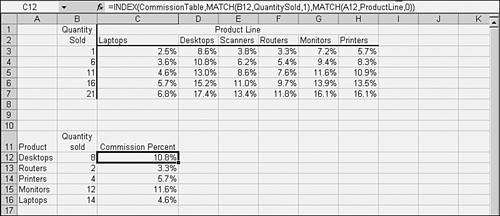
In Figure 3.11, as in Figure 2.9, the value in cell C12 is 10.8%. In Figure 2.9, the formula in C12 is based on the INDEX function, and it uses columns and rows as its arguments: =INDEX($C$3:$H$7,MATCH(B12,$B$3:$B$7,1), _ MATCH(A12,$C$2:$H$2,0))
That's not a formula that's rich in intuitive meaning. If you entered it on Monday and had another look at it on Friday, you'd spend a few seconds figuring out what it's intended to do. Now suppose that you define some names, so that The name CommissionTable refers to $C$3:$H$7. The name ProductLine refers to $C$2:$H$2. The name QuantitySold refers to $B$3:$B$7.
Notice that the ranges that the names refer to are the ranges used in the INDEX formula, repeated from Figure 2.9. But now those ranges have names, and you can use this formula as shown in Figure 3.11: =INDEX(CommissionTable,MATCH(B12,QuantitySold,1), _ MATCH(A12,ProductLine,0))
That's a lot easier to interpret. You can look at it and see almost at once that it returns from the commission table the value that is found at the intersection of a particular quantity and a particular product. There are several good methods you can use to define these names. The method shown next gives you the most control. Using the layout shown in Figure 3.11, follow these steps: - Choose Insert, Name, Define.
- In the Names in Workbook box, type CommissionTable.
- Click in the Refers To box and then, using the mouse pointer, drag through the worksheet range C3:H7. (Notice that when you use the worksheet in this way to establish a reference, Excel makes the reference absolute.)
- Click OK, or click Add if you're not through defining names.
Another convenient method to establish a named range involves the Name box. Begin by selecting the worksheet range C3:H7. Now click in the Name box that's the box with the drop-down arrow, at the left edge of the Excel window and on the same row as the Formula Bar. Type the name CommissionTable and then press Enter. Similarly, you could begin by selecting B3:B7, clicking in the Name box, typing QuantitySold, and pressing Enter. TIP The Name box is a convenient way to tell whether the active range or cell has a name and, if so, what the name is. After naming the QuantitySold range, for example, the Name box shows that name if you select the range B3:B7. Turning it around, you can choose a name from the Name box's dropdown in order to select that range on the worksheet.
The Name box displays only names that refer to worksheet cells and ranges, and you can use it to define only range and cell names. Using Implicit Intersections Suppose that you define the name Quantity as referring to the range B12:B16 in Figure 3.11. Now, select a cell in some column other than B, and in a row anywhere from 12 through 16, you enter this formula: =Quantity
That formula will return the corresponding value in the range named Quantity. For example, suppose that you entered that formula in cell F14. It would return the value 4: the value in the cell where the range named Quantity (that is, B12:B16) intersects the row where you enter the formula (here, row 14). That value is 4, so that's what the formula returns. This is an example of an implicit intersection. It's implicit because the row is implied by the location of the formula. If you entered the same formula in row 16, it would return the value 14, where row 16 intersects the range named Quantity. Suppose that the range that you name Quantity occupies several columns in one row, rather than several rows in one column. You enter the same =Quantity formula in one of its columns but in a row that's outside the named range. In that case, you would get the same effect: an implicit intersection, but with one of the range's columns instead of one of its rows. The implicit intersection is useful in the current example on sales commissions. If you give the name Quantity to the range B12:B16 in Figure 3.11, you can enter this formula in C12: =INDEX(CommissionTable,MATCH(Quantity,QuantitySold,1),MATCH(A12,ProductLine,0))
Note the difference from the earlier example. In the first MATCH, the argument B12 has been replaced with a reference to Quantity. Because you have entered it in cell C12, the implicit intersection picks up the value 8 from cell B12 and returns the original result, 10.8%. When you copy and paste that formula into C13:C16, the implicit intersection again gets the necessary values from B13:B16, and again returns the proper results. In the same way, you could give the name Product to the range in A12:A16. Then you could completely dispense with cell and range references: =INDEX(CommissionTable,MATCH(Quantity,QuantitySold,1), _ MATCH(Product,ProductLine,0))
Now the formula has become self-documenting. You need not go back and forth between cell references in the formula and their contents in the worksheet to figure out what's going on. NOTE If a formula that relies on an implicit intersection is entered outside the rows or columns that the named range occupies, the formula returns the #VAL! error.
Defining Static Range Names A name is static if it refers directly to a cell or range of cells. It's useful to distinguish a static name from a dynamic name, which refers to a range that can change size automatically as new data arrives (see the next section for more information). You've already seen a couple of ways to define static range names: using the Name box, and using Insert, Name, Define. You can also use the Create item in the Name menu. If you have an Excel list, you can easily create static range names based on the list's variable names. Select the entire list, choose Name from the Insert menu, and click Create. The window shown in Figure 3.12 appears. Figure 3.12. Filling the Left Column check box misleads Excel into treating the values Democrat and Republican as Names. 
By filling the Top Row check box and clicking OK, you create three names: the name Party refers to $A$2:$A$21, Sex refers to $B$2:$B$21, and Age refers to $C$2:$C$21. If your variable names are in the range's left column, instead of its top row, fill the Left Column check box. To create names that occupy rows as well as names that occupy columns, fill both the Left Column and the Top Row check boxes before clicking OK. The Create Names window even allows for eccentrically placed variable names: If you've put them in the rightmost column or bottommost row, just fill the appropriate check boxes. Defining Dynamic Range Names Dynamic names are those that change the dimensions of the ranges they refer to, depending on how much data the ranges contain. Figure 3.13 gives an example. Figure 3.13. Dynamic range names are effective in formulas and charts based on data that you update frequently. 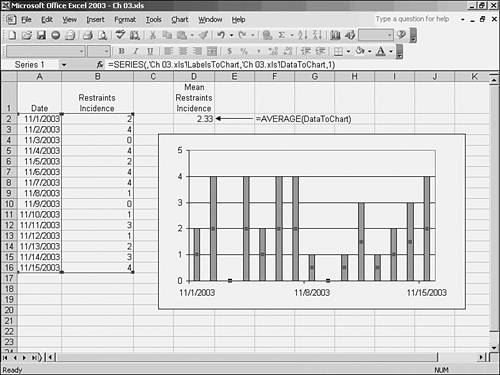
There are two named ranges in Figure 3.13: one named LabelsToChart and one named DataToChart. The name LabelsToChart refers to the date values in column A. These are dates on which observations were made. The name DataToChart refers to the counts in column B. These count the incidents of the use of restraints in a hospital on a given date. The user wants to know the average daily incidence of the use of restraints, and to chart the actual daily incidence over time. Both range names were defined by choosing Insert, Name, Define. This is the only way to define a dynamic range name; the Name box won't help you here. Here's the definition of the range LabelsToChart, as found in the Refers To box of the Define Names window: =OFFSET(Restraints!$A$1,1,0,COUNT(Restraints!$A:$A),1)
TIP The easiest way to enter this reference is to click in the Refers To box. Type =OFFSET( and then click in cell A1. Excel will put Restraints!$A$1 in the formula for you. When you get to the argument to the COUNT function, click the column label A. Excel automatically puts the reference Restraints!$A:$A into the formula.
This is another useful instance of the OFFSET function, already discussed in Chapter 2, "Excel's Data Management Features." In words, here's what it does: The COUNT function, as used in the name definition, returns the number of numeric values found in column A of the worksheet named Restraints. In the case shown in Figure 3.11, that result is 15. The 15 dates found in A2:A16 are all numbers, and the one label in cell A1 is a text value. The definition can now be simplified to =OFFSET(Restraints!$A$1,1,0,15,1)
Using the syntax of the OFFSET function, the definition refers to the range that's offset from $A$1 by one row and zero columns, that's 15 rows high and one column wide in other words, A2:A16.
Suppose now that you have reached November 16 on the calendar and it's time to enter another day's worth of data. You type 11/16/2003 in cell A17. Notice what happens to the definition of the dynamic range name LabelsToChart: The COUNT function in the definition now finds 16, not 15, numeric values in column A. So the definition now refers to the range that's offset from $A$1 by one row and zero columns, that's 16 rows high and one column wide that is, A2:A17. This is why the name is termed a dynamic range name. The COUNT function makes it sensitive to the number of numeric values in column A. The more values in that column, the more rows in the named range. The other named range in Figure 3.13, DataToChart, is defined as =OFFSET(LabelsToChart,0,1)
in the Define Names window's Refers To box. This makes the name dependent on the name LabelsToChart: It is offset from that range by zero rows and one column. Because the (optional) height and width arguments are not provided, the DataToChart range automatically assumes the same number of rows and columns as LabelsToChart. So, as the number of rows in LabelsToChart increases (or decreases), so does the number of rows in DataToChart. After all this hand-waving, you're in a position to take advantage of the dynamic range names. In cell D2 of Figure 3.13, you find the formula =AVERAGE(DataToChart), which with the data as shown in column B returns the value 2.33. Suppose that you now enter 11/16/2003 in cell A17 and 4 in B17. This increases the average restraints incidence from 2.33 to 2.44. It also causes both ranges to increase by one row, and the formula =AVERAGE(DataToChart) recalculates accordingly. Another effect appears in the chart. An additional column appears on the chart to reflect the new values entered in A17:B17. This is because the charted series is defined in the chart as =SERIES(,'Ch 03.xls'!LabelsToChart,'Ch 03.xls'!DataToChart,1)
TIP To view or edit what a chart's data series refers to, click on the series to select it. You can then see what it refers to, and edit that information, in the Formula Bar.
So, as each range gets more data, the names are dynamically redefined to capture the new information, and the chart updates to show more labels on its x-axis and more values in its columns. There are a couple of aspects to dynamic range names that it pays to keep in mind, and we'll discuss them in the following sections. Looking Out for Extraneous Values Notice in Figure 3.13 that the formula =AVERAGE(DataToChart) is outside column A. If it were in column A, it would count as a numeric value, and would contribute to the number of numeric values returned by the COUNT function in the definition of LabelsToChart. Suppose, for example, that =AVERAGE(DataToChart) were in column A. Then =AVERAGE(DataToChart) would involve a circular reference: The formula would contribute to the definition of the range it refers to. (There are situations in which this can be a good thing, but this isn't one of them.) Or suppose that you somehow let an extraneous numeric value get into column A as far away, perhaps, as cell A60000. Then column A would have 15 dates and one extra, unwanted number, each counting as a numeric value. The COUNT function would return 16, not 15, and LabelsToChart would extend from A2:A17. To use dynamic range names effectively, you need to make sure to keep extraneous values out of the range that COUNT looks at. Selecting Dynamically Defined Ranges Static range names are available in the Name box: You can click the Name box's dropdown and choose a range name to select that range. They're also available via the Go To item in the Edit menu. The list box shows all accessible range names; just select one of them and then click OK to select its range. Dynamic range names don't behave that way. You'll never see one in the Name box not, at least, through the 2003 version of Excel. And if you choose Go To from the Edit menu, you won't see dynamic range names in the list box. You can, however, choose Go To from the Edit menu, and type an already existing dynamic range name in the Reference box. When you click OK, Excel selects the range that's currently defined by that dynamic name. Understanding the Scope of Names Names can be either workbook-level or worksheet-level names. Workbook-level names are the default, and are the type that this chapter has discussed so far. Workbook-level names (often referred to more briefly as book-level names) are accessible from any worksheet or chart sheet in a workbook. So, if the book-level name DataToChart refers to a range on Sheet1, you can use that name in any sheet in the workbook. For example, the formula =AVERAGE(DataToChart) could be used on Sheet2 or Sheet3, and would return the same result each time. You define a book-level name using any of the methods discussed so far in this chapter: by means of the Name box, using the Define Names dialog box, or with the Create Names dialog box. One possible drawback to a book-level name is that only one instance of that name can exist in a workbook. For example, you can't use the book-level name DataToChart to refer to A1:A20 on Sheet1 and also to some other range, such as C1:C20 on Sheet1, or A1:A20 on Sheet2, or to a constant or a formula. A book-level name can exist only once in a workbook and can have one reference only. In contrast, a worksheet-level name (also termed a sheet-level name) can exist once in a workbook for each sheet in that workbook. One sheet-level name DataToChart can exist for Sheet1, and another sheet-level name DataToChart can exist for Sheet2, and so on. Here's how to define the sheet-level name DataToChart for Sheet1 and Sheet2 (you can extend it to as many worksheets as you like): - Activate Sheet1.
- Choose Insert, Name, Define.
- In the Names in Workbook box, type Sheet1!DataToChart.
That is, qualify the range name by the name of the worksheet it is to belong to. Separate the name of the worksheet from the range name itself with an exclamation point.
- In the Refers To box, assign whatever reference you want: a constant, formula, or worksheet range. (If you cause the name to refer to a worksheet range, bear in mind that you can choose a range on any worksheet not just Sheet1. That is, the name Sheet1!DataToChart can refer to B1:B10 on Sheet2.)
- Click OK, or click Add to continue defining names.
You could also use the Name box: Select the range you want to refer to, then type, for example, Sheet1!DataToChart in the Name box. When you're through entering sheet-level names, it's a good idea to double-check them in the Define Names window (see Figure 3.14). Figure 3.14. Which sheet-level names are visible depends on which sheet is active when you choose Insert, Name, Define. 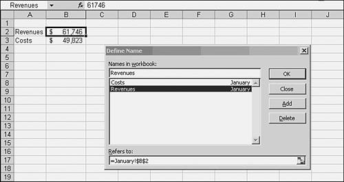
Notice that the name of the sheet to which the name belongs (in Figure 3.14, that's January) appears to the right of the sheet-level name in the Names in Workbook list box. Sheet-level names are very handy when you assign similar kinds of data to different sheets in a workbook. For example, you might place a different income statement for each month in a year on a different worksheet. Each worksheet might be named according to its month. Then, you could have January!Revenues, February!Revenues, March!Revenues, and so on. Keep these points in mind as you work with sheet-level names: You don't need to qualify a sheet-level name when you use it on the sheet that it's defined for. That is, if the worksheet named January is active, the formula =SUM(Revenues) is equivalent to =SUM(January!Revenues). If you want to refer to a sheet-level name, and the sheet that it's defined for is not active, you must qualify the name. If the February worksheet is active, and you want it to show the sum of January's revenues, you would need to enter =SUM(January!Revenues). This is true even if there is no sheet-level name February!Revenues.
|