| The last section discussed one way to manage arrays of data using INDEX along with MATCH. Another closely related technique uses VLOOKUP. Unlike MATCH, VLOOKUP returns a value, not a position in a range, so it's seldom necessary to pair VLOOKUP with a function such as INDEX. As a practical matter, VLOOKUP requires a range of at least two columns, but you often use it to return a value from a range with three or more columns. The distinction is similar to one you've just seen. Compare Figure 2.6 (two columns: one for quantity and one for percentages) with Figure 2.9 (seven columns: one for quantity and six for percentages). Using VLOOKUP with a Two-Column Range To use VLOOKUP with a two-column range, you need lookup values in the first column, just as with MATCH combined with INDEX. Similarly, the second column should contain the values you want it to return. Figure 2.10 gives an example. Figure 2.10. VLOOKUP is usually more convenient than MATCH when just two columns are involved. 
It's useful to assign terms to VLOOKUP's arguments: VLOOKUP's first argument is the lookup value. It is the value that VLOOKUP will look for. It can be an actual value, a cell address, or even a defined name. VLOOKUP'S second argument is the lookup array. It is a range of at least one column and one row; normally, the lookup array contains two or more columns and at least several rows. VLOOKUP's third argument is the column number. It is the column that VLOOKUP uses to find the value it returns. VLOOKUP's fourth argument is the lookup type. As in MATCH, it tells Excel whether to make an exact or an approximate match.
In Figure 2.10, the VLOOKUP function is used instead of INDEX and MATCH, which were used in Figure 2.6. In Figure 2.10, the formula in cell B12 is =VLOOKUP(A12,$A$3:$B$7,2,TRUE)
The process works as described in the following list: VLOOKUP is asked to find the value in A12, the lookup value. VLOOKUP always looks in the first column of the lookup array to find a matching value. The lookup array is in $A$3:$B$7; the first column in the array is column A, so that's where VLOOKUP searches for a matching value--more specifically, in A3:A7. After the value in A12 has been found in A3:A7, VLOOKUP needs to know which column to return. The column number argument (here, the value 2) provides that. In the example, VLOOKUP is asked to return the value in the second column of the lookup array. The fourth argument tells VLOOKUP whether to find an exact or an approximate match in the lookup array. Here the value TRUE specifies an approximate match, looking for the largest value that's less than or equal to the lookup value. This is the same as in the MATCH function, except that VLOOKUP uses TRUE where MATCH uses 1. The TRUE in VLOOKUP and the 1 in MATCH are the defaults.
VLOOKUP looks for the value 14 in the first column of the range A3:B7. Because the lookup type specifies an approximate match, VLOOKUP uses 11: the third value in the first column and the largest value that is less than or equal to 14. VLOOKUP then looks in the second column of the lookup array, as specified by the column number argument. In the lookup array's third row, second column is the value 4.6%, which is the value that VLOOKUP returns. You'll probably find VLOOKUP more convenient than the combination of MATCH and INDEX for lookup arrays with only two columns. It's not quite as clear what's going on because it's not intuitively obvious that VLOOKUP always looks to the first column of the lookup array to find a matching value. But it is nice to take advantage of VLOOKUP's brevity: You need only one function instead of two. CASE STUDY
Calculating Commissions with VLOOKUP As the sales manager for a local distributor of computing equipment, Debra Brown wants to guide her sales force toward sales that involve more units. Selling one desktop here and a couple of routers there is well and good, but the fulfillment costs eat into the profit margins. Brown would prefer one sale of five monitors, for example, to seven sales of one monitor each. Accordingly, she draws up a commission schedule that gradually increases the commission percentage according to the number of units sold. The percentages vary both by product line and by quantity sold. Her table of commission percentages is shown in cells C2:H7 of Figure 2.11. Figure 2.11. If you have more than two columns in the lookup array, you're probably back to requiring MATCH. 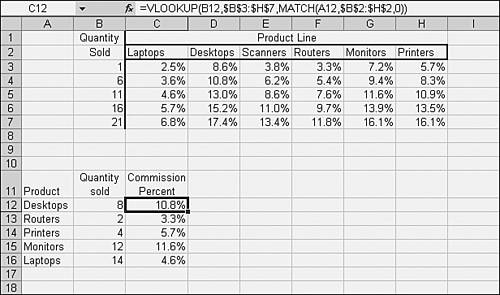
After setting up the table, Brown starts to enter VLOOKUP formulas to determine actual commission dollars. She encounters a typical problem: VLOOKUP is less convenient when you're working with more than two columns than it is when you're working with exactly two. The problem with multiple columns is to get the correct column number into the VLOOKUP arguments. NOTE It will become clear that the sales manager could use a combination of MATCH and INDEX in this case study, just as was shown in Figure 2.9, instead of VLOOKUP. The choice is largely a matter of style and personal preference. Your formulas are somewhat more explicit when you go to the trouble of passing the results of MATCH functions to INDEX. But they are also inevitably lengthier, and many expert users prefer the terser VLOOKUP syntax to the more verbose MATCH-INDEX combination.
In Figure 2.11, cell C12 is intended to show the commission percentage for selling some number of Desktops. VLOOKUP is able to figure out which row in the lookup table to use: It finds that 6 is the largest value that's less than or equal to the lookup value. But VLOOKUP doesn't automatically know which column to use--it's up to the user to give it that information. Unless the situation is simple enough that you can get by with constants such as 2, 3, and 4 for the column number, you need a way to identify the column to use. In Figure 2.11, Ms. Brown has used the MATCH function to find the column, just as was done in the earlier section on MATCH and INDEX in two-way arrays. The formula is =VLOOKUP(B12,$B$3:$H$7,MATCH(A12,$B$2:$H$2,0))
The MATCH function looks for the value in A12, Desktops, in the range $B$2:$H$2. It finds Desktops in the third position of that array, so the VLOOKUP function simplifies to this: =VLOOKUP(B12,$B$3:$H$7,3)
Compare the VLOOKUP approach with the INDEX and MATCH approach; to review, you use INDEX and MATCH in this way: =INDEX($C$3:$H$7,MATCH(B12,$B$3:$B$7,1),MATCH(A12,$C$2:$H$2,0))
There's no question that the VLOOKUP approach is a little more concise, and many users prefer it. Others prefer the INDEX and MATCH approach because it makes what's going on a little clearer--you match one value to get a row, another to get a column, and return their intersection. As you become familiar with using Excel functions to locate data, you're likely to develop your own preference. Brown completes the formulas needed to determine the applicable percentage for a given quantity in a product line and enters them in cells C12:C16. She still has to determine the actual dollar amounts, and that's simple compared to determining the commission percentage. Brown enters a new table, shown in cells J2:K6 of Figure 2.12, to associate a sales price with each product. She picks up the product price using a combination of MATCH and INDEX, and then multiplies the quantity in column B times the percentage in column C times the price. That formula appears in cell D12 of Figure 2.12. Figure 2.12. This is a good opportunity to use range names, discussed in Chapter 3, in place of absolute addressing. 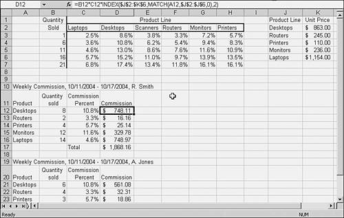
|