| You probably won't have much use for the MATCH function all by itself. Think back: How often have you wondered where to find the number 5 in the range C10:C100 by means of a worksheet function? But when you use MATCH as an argument to another function, such as INDEX or OFFSET, you begin to appreciate how valuable it is. Combining MATCH and INDEX That aspect of MATCH--being able to find the largest value less than or equal to the value you're looking for--is useful when you have to deal with grouped values as seen in Figure 2.6. Figure 2.6. Consider using MATCH whenever several values (such as 11 through 15) are associated with one value (such as 4.6%). 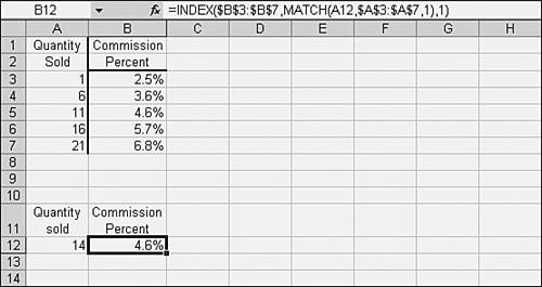
In Figure 2.6, the user is looking for the proper commission rate to pay for a sale of 14 items. The proper rate is 4.6%: the rate that applies when 11, 12, 13, 14, or 15 units are sold. You get that rate by looking for the right group of units by means of MATCH, and then using MATCH's result to find the value you're after. The formula shown in Figure 2.6 is =INDEX($B$3:$B$7,MATCH(A12,$A$3:$A$7,1),1)
Look first at the MATCH part of the formula: MATCH(A12,$A$3:$A$7,1)
This tells Excel to look for the value in A12 (which is 14) in the range $A$3:$A$7, and return the position of the largest value that's less than or equal to 14 (the third argument to MATCH, 1, calls for the less-than or equal-to approximate match). The value 11 is the largest value that's less than or equal to 14 in $A$3:$A$7, and it's in position number 3 in that range. So, MATCH returns the value 3. In the original formula =INDEX($B$3:$B$7,MATCH(A12,$A$3:$A$7,1),1)
you could replace the MATCH function and its arguments with 3, the value it returns, as follows: =INDEX($B$3:$B$7,3,1)
So, by using MATCH to approximately locate the value 14, you tell INDEX to return the value in the third row, first column of $B$3:$B$7, or 4.6%. TIP If you're using Excel 97 or 2000, you can select a cell containing a formula such as the one discussed here, and in the Formula Bar, use your mouse pointer to drag across some portion of it, such as MATCH(A12,$A$3:$A$7,1). Then press the F9 key to see how Excel evaluates the highlighted portion. Press Esc to leave the formula as is. (If you press Enter, you might unintentionally convert the highlighted portion to a constant.) If you're using Excel 2002 or 2003, you can do the same thing, but instead you can choose Tools, Formula Auditing, Evaluate Formula to see, step by step, how Excel evaluates each portion of the formula.
The following list outlines the main points you need to remember: Make sure that the array (in Figure 2.6, that's B3:B7) is in ascending order. This is because you will call for an approximate match. To call for the approximate match, use 1 as MATCH's third argument. Make sure to convert the position (what MATCH actually returns) to a value (what you're really after). In many cases, including this one, that means passing the result of the MATCH function as an argument to the INDEX function.
TIP This way of using functions--that is, using the result of one function as an argument to another--has broad applicability in Excel, particularly in the text functions. For example, you could get an email address stripped of its domain with something such as =LEFT(D1,FIND("@",D1)-1)
Fooling the Approximate Match It's not unusual to use functions and their arguments in ways that they weren't originally intended. One good example involves MATCH, OFFSET, and the MAX function. The MAX function returns the largest numeric value in a range. For example, this formula =MAX(A1:C200)
returns the largest value in A1:C200. Suppose that you want to know the location of the final value in, say, Column A. One way to do that is to activate cell A65536, the final cell in Column A. Hold down the Ctrl key and press the up arrow key. Assuming that A65536 is an empty cell, this will take you to the bottommost nonempty cell in Column A. NOTE This chapter makes frequent use of the terms bottommost and rightmost, so it's good to define them, if only by example. Suppose that column A has the value 8 in row 25 and nothing at all in rows 26 through 65536. In that case, A25 is column A's bottommost cell. If row 4 has the value "EBCDIC" in column AD and nothing at all in columns AE through IV, AD4 is row 4's rightmost cell.
Fine, but that's not very convenient, especially if there are several columns of interest. And if you want to use the last value in a column in another formula, you want to be able to redetermine that value as more cells are filled in. Further, you might want to test whether some extraneous value has found its way into a column, well below the area where your work normally occurs. A fairly ingenious use of the approximate match solves the problem (see Figure 2.7). Figure 2.7. This technique does not work with text values. 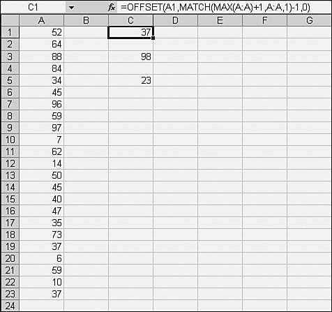
The formula in cell C1 of Figure 2.7 is =OFFSET(A1,MATCH(MAX(A:A)+1,A:A,1)-1,0)
and it returns 37, the last (bottommost) value in column A. This would normally be a trivial usage because you can see it. But suppose that the last value were in cell A4500, where it wouldn't be quite so obvious. Or suppose that the formula returned 2432, against your expectations. That would cue you to look further to see how that 2432 value got in there. To see what's going on, take the formula apart. Cell C3 contains this fragment from the complete formula =MAX(A:A)+1
which returns 98. The value 97 is the largest value in column A, and adding 1 to it results in 98. Substituting that value for the MAX function in the complete formula leaves this: =OFFSET(A1,MATCH(98,A:A,1)-1,0)
Now, what does the MATCH function return? This fragment is in cell C5 =MATCH(98,A:A,1)
and it returns the value 23. As you've seen, the value 1 as MATCH's third argument requests the largest value in the lookup range that is less than or equal to the lookup value. Here, though, the MATCH function is confronted with a lookup value that is larger than any value in the lookup range. It has to be, because it's the result of adding 1 to the maximum value in the range. Because the lookup type of 1 promises that the range is in ascending order, MATCH locates the range's final value: According to the promise of an ascending sort, that's its largest value. By using one more than MAX as the lookup value, the final value must be less than or equal to the lookup value. So, the MATCH function returns the position of that final value; here, that's 23. Notice that if you wanted to, you could stop at this point. You might do that if you were interested less in the actual value than in where it's located. You already know that the final value is in the 23rd position of the lookup range (which is Column A). But if you want to know the value itself, take one more step. Here are two versions of the original formula, simplified by using the results of the MAX and the MATCH functions: =OFFSET(A1,23-1,0)
or =OFFSET(A1,22,0)
That is, the value that is 22 rows below and zero columns to the right of A1, and that's 37. TIP A good way to test your understanding of the material in this section is to change the original formula so that it searches for the rightmost value in a row, rather than the bottommost value in a column. If you do, remember to switch the position of the row and column arguments in the OFFSET function. Also, bear in mind that while you refer to the first column as A:A, you refer to the first row as 1:1.
Extending the Last Cell Search The technique described in the prior section is fine for single columns and single rows, but what about a full range such as A1:G200? And what about text values, which the MAX function isn't able to locate? Figure 2.8 demonstrates one approach, attributed to Bob Umlas. To show the idea in book format, the range that contains values is kept small, A1:G20, although the range actually searched is much larger, A1:G500. Of course, if you use this in your own work, the range that contains values is likely to be much larger. Figure 2.8. If these formulas were entered normally, they would return the #VALUE! error value. 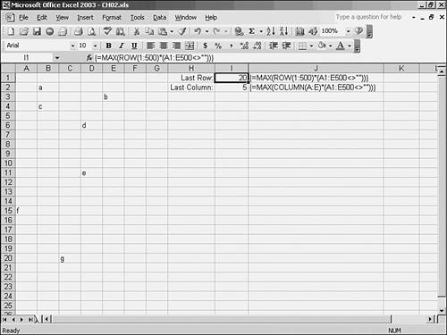
The formula in J1 of Figure 2.8 is {=MAX(ROW(1:500)*(A1:E500<>""))}
Note the curly braces indicating an array formula. Excel adds them automatically when you array-enter a formula with Ctrl+Shift+Enter instead of pressing just the Enter key. The formula in J1 returns 20, the row in which the bottommost value in the range A1:E500 is found. It's helpful to parse the formula to better understand how it works. This portion ROW(1:500)
returns an array of row numbers, separated by semicolons (recall that Excel separates row references by semicolons and column references by commas). It looks like this: {1;2;3;4; ... ;499;500}
Or it would if you could see it all. NOTE Using the Excel 97 and 2000 technique, dragging across ROW(1:500) to highlight it in the Formula Bar and then pressing F9 results in the message that the formula is too long. The Excel 2002 and 2003 technique, using the Formula Evaluator, does not result in an error, but returns a single value only when applied to the ROW(1:500) expression.
So far, the formula has created an array of 500 row numbers. The next portion is (A1:E500<>"")
It returns this array {FALSE,FALSE,FALSE,FALSE,FALSE;FALSE,TRUE,FALSE,FALSE,FALSE; . . .;}
which shows FALSE if a cell equals "" (that is, the cell contains a blank), and TRUE if a cell does not equal '''' (so, the cell contains anything other than a blank, including numbers and text, but not error values such as #REF!). Notice that the first five values in the array are separated by commas. They represent cells A1:E1, which are in different columns but in the same row, so they are separated by commas. The first through fifth values and the sixth through tenth values are separated by a semicolon. Collectively, they represent A1:E1 and A2:E2, which are in different rows, so the first five are separated by a semicolon from the second five. Also notice that the seventh value in the array is TRUE. This corresponds to cell B2, which Figure 2.8 shows to contain the value a. It's not a blank cell, so the formula returns a TRUE. By now two portions of the formula have been evaluated, and we have an array of numbers from 1 through 500, and an array of TRUE or FALSE values. The original formula calls for those two portions to be multiplied together. When you multiply the value TRUE times a number, the result is that number. So, 7*TRUE equals 7. When you multiply the value FALSE times a number, the result is 0. Multiplying the two arrays together, then, returns 0s where the cell contains a blank (and so the second array contains a FALSE). It returns the row number from the first array when the cell contains a nonblank, nonerror value (the row number times TRUE gives the row number). Here's what the first part of the array looks like: {0,0,0,0,0;0,2,0,0,0;
Notice that the array contains 0s where the cell is blank, and the cell's row number where the cell is neither blank nor an error. In the fragment shown above, the row number is 2. By now ,the formula has returned an array consisting of 0s and the numbers of rows that contain values. By applying MAX to the result, it's possible to learn the largest value in that array: the largest row number in the range that contains a legitimate value. Substituting the prior array for the formula fragments that create it =MAX({0,0,0,0,0;0,2,0,0,0; . . . ,0;})
returns what the formula's after: the bottommost row in a multi-column range that contains a legitimate value. Of course, the formula in cell J2 works in much the same way, except that it deals with the maximum column number instead of the maximum row number. Distinguishing the Bottommost Cell from the Last Cell There's a subtle difference between what the prior two sections have meant by the term bottommost cell (and rightmost cell) and what Excel means by last cell. As used in this chapter, the bottommost cell is the one that contains a value and that is farthest down the worksheet--that is, the value that occupies the row with the largest row header. By last cell, Excel means the bottommost, rightmost cell that has been used since the workbook was last saved. The phrase has been used needs some clarification. The following actions are all considered using a cell: Entering a value in a cell Formatting a cell, even an empty one Changing a row's height or a column's width Changing a cell's protection--for example, from locked to unlocked
One implication of this is that an empty cell could be considered the last cell. To demonstrate this to yourself, take the following steps: - Open a new workbook.
- Select some cell other than A1, such as E5.
- Choose Format, Cells and click the Number tab. Give the cell any format other than General--in other words, change the cell's default format.
- Select cell A1.
- Choose Edit, Go To and click the Special button. Fill the Last Cell option and click OK. Excel selects the cell you formatted.
This definition of last cell is not the same as that used in the prior two sections, where a bottommost or a rightmost cell was defined by the presence of a value in the cell. And it's more persistent as well. Clear a value from the bottommost cell in Column A, for example, and the formula =OFFSET(A1,MATCH(MAX(A:A)+1,A:A,1)-1,0)
no longer displays that value. Rather, it displays the new bottommost value. In contrast, click the Select All button on the worksheet you used to test for the location of its last cell, and choose Edit, Clear, All. Even though you've reset the format of all the worksheet's cells to General, you still activate the same last cell by means of Edit, Go To, Special, Last Cell. You force Excel to redefine the last cell by closing the workbook (saving changes) and then reopening it. No matter whether you enter and then clear a value from a cell, or format and then clear the format from a cell, or reset the row height or column width, Excel continues to activate that cell as the last cell until you close and then reopen the workbook. Using MATCH and INDEX in Two-Way Arrays Figure 2.9 extends the example, begun in Figure 2.6 and implying one product line only, to several product lines. Figure 2.9. Here you use MATCH to find both the proper row and the proper column. 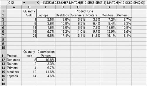
Figure 2.9 shows that MATCH works with both numeric and text values. As shown, the formula in cell C12 is =INDEX($C$3:$H$7,MATCH(B12,$B$3:$B$7,1),MATCH(A12,$C$2:$H$2,0))
Again, break the formula down into its components. The first instance of MATCH is MATCH(B12,$B$3:$B$7,1)
That is, return the position occupied in $B$3:$B$7 by the largest value that's less than or equal to the value in B12. B12 contains 8, and the largest value in $B$3:$B$7 less than or equal to 8 is 6. The value 6 occupies the second position in $B$3:$B$7, so this instance of MATCH returns 2. The second instance of MATCH is MATCH(A12,$C$2:$H$2,0)
That is, return the position occupied in $C$2:$H$2 by the value in A12, and return an exact match. (The third argument, 0, calls for an exact match.) The value in A12 is Desktops, and Desktops occupies the second position in $C$2:$H$2. So, this instance of MATCH also returns 2. NOTE The reason that the second instance of MATCH calls for an exact match is that approximate matches are seldom sensible with text values. In Figure 2.9, for example, you would not want MATCH to return Scanners if you had it look for Software.
To see more clearly what's happening in the full formula, replace the two MATCH functions with the values they return. Again, you can do this by dragging across MATCH(B12,$B$3:$B$7,1) in the Formula Bar and pressing F9. Follow that up, if you wish, by doing the same with MATCH(A12,$C$2:$H$2,0). Or in Excel 2002 or 2003, use Tools, Formula Auditing, Evaluate Formula. When you do so, the INDEX function simplifies to this: =INDEX($C$3:$H$7,2,2)
In words, return the value in the second row and second column of the range $C$3:$H$7. That value is 10.8%, which is the commission rate indicated for selling eight desktops. When you use MATCH in this way, it's not necessary that the range you're looking in to find the proper row occupy the same rows as the values you want to return. For example, the range $B$3:$B$7, with the quantity sold, could just as easily be in $GW$200:$GW$204 and the actual commission percentages could stay in $C$3:$H$7. But it's a lot easier to arrange your data as Figure 2.9 shows. NOTE This chapter hasn't mentioned it yet because it's so seldom used, but the lookup type argument to the MATCH function has another possible value. This chapter has examined the effect of 0 (return an exact match) and of 1 (return an approximate match, the largest one that's less than or equal to the lookup value in an array that's sorted in ascending order). A third possibility is 1, and it also requests an approximate match: find the smallest one that's greater than or equal to the lookup value in an array that's sorted in descending order. It takes an idiosyncratic data layout to require this approach, but bear in mind that it's available if you ever encounter one.
|