| Excel is not a database management system. It is not, for example, designed to manage the relationship between parent and child records. To extend the example in the previous section, a PO is a parent record and invoices are child records because each invoice the child record belongs to a PO the parent record. Still, Excel has some rudimentary database features, among them the AutoFilter and the Advanced Filter. These two filters in particular depend on a particular orientation of your data, called lists. In Excel, a list has these characteristics: Each record (each person, each product, each invoice) occupies a different row. Each variable (for example, name and address, or model and price, or invoice date and amount) occupies a different column. Each column begins with the name of the variable that's located in that column.
Figure 1.1 is an example of a list. It has different records invoices in different rows, different variables dates, amounts, and so on in different columns, and each column is headed by the name of that column's variable. Changing the Orientation with Paste Special Many of Excel's tools work best, and some work only, when the data you point them at are arranged in lists. Tools such as pivot tables and data filters will not work properly with any other arrangement. From time to time, a user might decide to enter data using a different layout. When this happens, it's often a 90-degree rotation from the normal list arrangement; that is, he puts different records in different columns and different variables in different rows. Figure 1.6 shows an example. Figure 1.6. A user might lay out his data this way for any reason from aesthetics to lack of experience with list structures. 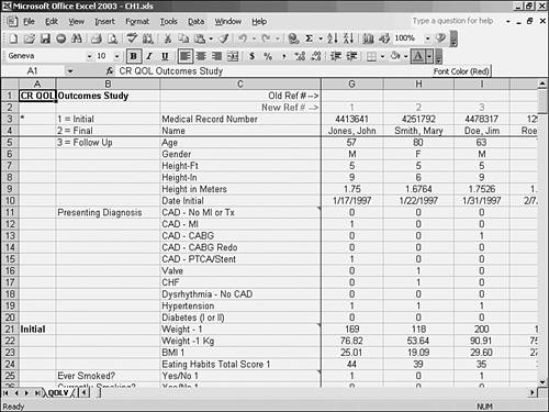
This arrangement is unwise for several reasons, but the strongest is that the user will run out of columns long before he runs out of rows. An Excel worksheet has 256 columns only, and there's no way to add more. But it has 65,536 rows. (No, you can't add more rows either, but 65,536 is pretty roomy. 65,536 is 2 to the 16th power, by the way.) There are many situations in which you would have more than 256 records. For example, a company of any appreciable size has more than 256 invoices to deal with. But it is rare to have as many as 256 variables that describe the records. So, the dimensions of the worksheet itself argue for using the list structure. Nevertheless, you frequently encounter worksheets laid out as in Figure 1.6. If only a few formulas are based on the data as it's shown in the figure, there are a couple of easy fixes: - Select the entire data range.
- Choose Copy from the Edit menu.
- Select a cell that has empty columns to its right.
- Choose Paste Special from the Edit menu, fill the Transpose check box, and click OK.
- Repair the range addresses used in the formulas.
CAUTION Be careful when transposing data using Paste Special. In some cases, you can transpose formulas so that they depend on cells that don't exist. Chapter 2 discusses this problem in detail.
Changing the Orientation with the TRANSPOSE Function Sometimes the user has structured the worksheet as shown in Figure 1.6 because it's easier to enter the data that way perhaps the data comes in a hardcopy format with records in columns and variables in rows. Then it's much easier on the person entering the data to follow the arrangement of the hard copy. To preserve the data entry format and yet reconfigure the data so that it forms a list, you could take these steps: - Count the number of rows and columns in the existing data range.
- Select an entire range of blank cells. This new range should have as many columns as the original range has rows, and as many rows as the original range has columns.
- In the Formula Bar, type =TRANSPOSE( followed by the address of the original range (for example, A1:Z5), and a closing parenthesis.
- Array-enter the formula using the key combination Ctrl+Shift+Enter.
Now you have two ranges: One is laid out as in Figure 1.6, where more data can be entered as it becomes available, and the other appears as in Figure 1.7. Figure 1.7. The data seen in Figure 1.6 has been transposed and is now ready for analysis. 
To accommodate more records as they're entered into the original range, just select more rows in the new range before you enter the TRANSPOSE formula. That way, as more records are entered in columns in the original range, they'll appear in new rows in the transposed range. |