Section 7.5. Aggregating Values from Trees
7.5. Aggregating Values from TreesNow that you know how to deal with trees, let's look at how you can aggregate values held in tree structures. Most cases for the aggregation of values held in hierarchical structures fall into two categories: aggregation of values stored in leaf nodes and propagation of percentages across various levels in the tree. 7.5.1. Aggregation of Values Stored in Leaf NodesIn a more realistic example than the one used to illustrate the Vandamme and Highlanders queries, nodes carry informationespecially the leaf nodes. For instance, regiments should hold the number of their soldiers, from which we can derive the strength of every fighting unit. 7.5.1.1. Modeling head countsIf we take the same example we used previously, restricting it to a subset of the French Third Corps of General Vandamme and only descending to the level of brigades, a reasonably correct representation (as far as we can be correct) would be the tables described in the following subsections. UNITS. Each row in the units table describes the various levels of aggregation (army corps, division, brigade) as in tables adjacency_model, materialized_path_models, or nested_sets_model, but without any attribute to specify how each unit relates to a larger unit: ID NAME COMMANDER -- -------------------------- ----------------------------------------------- 1 III Corps Général de Division Dominique Vandamme 2 8th Infantry Division Général de Division Baron Etienne-Nicolas Lefol 3 1st Brigade Général de Brigade Billard 4 2nd Brigade Général de Brigade Baron Corsin 5 10th Infantry Division Général de Division Baron Pierre-Joseph Habert 6 1st Brigade Général de Brigade Baron Gengoult 7 2nd Brigade Général de Brigade Baron Dupeyroux 8 11th Infantry Division Général de Division Baron Pierre Berthézène 9 1st Brigade Général de Brigade Baron Dufour 10 2nd Brigade Général de Brigade Baron Logarde 11 3rd Light Cavalry Division Général de Division Baron Jean-Simon Domont 12 1st Brigade Général de Brigade Baron Dommanget 13 2nd Brigade Général de Brigade Baron Vinot 14 Reserve Artillery Général de Division Baron Jérôme Doguereau Since the link between units is no longer stored in this table, we need an additional table to describe how the different nodes in the hierarchy relate to each other. UNIT_LINKS_ADJACENCY. We may use the adjacency model once more, but this time links between the various units are stored separately from other attributes, in an adjacency list, in other words a list that associates to the (technical) identifier of each row, id, the identifier of the parent row. Such a list isolates the structural information. Our unit_links_adjacency table looks like this: ID PARENT_ID ---------- ---------- 2 1 3 2 4 2 5 1 6 5 7 5 8 1 9 8 10 8 11 1 12 11 13 11 14 1 UNIT_LINKS_PATH. But you have seen that an adjacency list wasn't the only way to describe the links between the various nodes in a tree. Alternatively, we may as well store the materialized path, and we can put that into the unit_links_path table: ID PATH ---------- ----------------- 1 1 2 1.1 3 1.1.1 4 1.1.2 5 1.2 6 1.2.1 7 1.2.2 8 1.3 9 1.3.1 10 1.3.2 11 1.4 12 1.4.1 13 1.4.2 14 1.5 UNIT_STRENGTH. Finally, our historical source has provided us with the number of men in each of the brigadesthe lowest unit level in our sample. We'll put that information into our unit_strength table: ID MEN ---------- ---------- 3 2952 4 2107 6 2761 7 2823 9 2488 10 2050 12 699 13 318 14 152 7.5.1.2. Computing head counts at every levelWith the adjacency model, it is typically quite easy to retrieve the number of men we have recorded for the third corps; all we have to write is a simple query such as: select sum(men) from unit_strength where id in (select id from unit_links_adjacency connect by prior id = parent_id start with parent_id = 1) Can we, however, easily get the head count at each level, for example, for each division (the battle unit composed of two brigades) as well? Certainly, in the very same way, just by changing the starting pointusing the identifier of each division each time instead of the identifier of the French Third Corps. We are now facing a choice: either we have to code procedurally in our application, looping on all fighting units and summing up what needs to be summed up, or we have to go for the full SQL solution, calling the query that computes the head count for each and every row returned. We need to slightly modify the query so as to return the actual head count each time the value is directly known, for example, for our lowest level, the brigade. For instance: select u.name, u.commander, (select sum(men) from unit_strength where id in (select id from unit_links_adjacency connect by parent_id = prior id start with parent_id = u.id) or id = u.id) men from units u It is not very difficult to realize that we shall be hitting again and again the very same rows, descending the very same tree from different places. Understandably, on large volumes, this approach will kill performance. This is where the procedural nature of connect by, which leaves us without a key to operate on (something I pointed out when I could not get rid of duplicates without destroying the order I wanted), leaves us no other choice than to adopt procedural processing when performance becomes a critical issue; "for all they that take the procedure shall perish with the procedure." We are in a slightly better position with the materialized path here, if we are ready to allow a touch of black magic that I shall explain in Chapter 11. I have already referred to the explosion of links; it is actually possible, even if it is not a pretty sight, to write a query that explodes unit_links_path. I have called this view exploded_links_path and here is what it displays when it is queried: SQL> select * from exploded_links_path; ID ANCESTOR DEPTH ---------- ---------- ---------- 14 1 1 13 1 2 12 1 2 11 1 1 10 1 2 9 1 2 8 1 1 7 1 2 6 1 2 5 1 1 4 1 2 3 1 2 2 1 1 4 2 1 3 2 1 7 5 1 6 5 1 10 8 1 9 8 1 13 11 1 12 11 1 depth gives the generation gap between id and ancestor. When you have this view, it becomes a trivial matter to sum up over all levels (bar the bottom one in this case) in the hierarchy: select u.name, u.commander, sum(s.men) men from units u, exploded_links_path el, unit_strength s where u.id = el.ancestor and el.id = s.id group by u.name, u.commander which returns: NAME COMMANDER MEN -------------------------- -------------------------------------- ----- III Corps Général de Division Dominique Vandamme 16350 8th Infantry Division Général de Division Baron Etienne- 5059 Nicolas Lefol 10th Infantry Division Général de Division Baron Pierre 5584 Joseph Habert 11th Infantry Division Général de Division Baron Pierre 4538 Berthézène 3rd Light Cavalry Division Général de Division Baron Jean-Simon 1017 Domont (We can add, through a union, a join between units and unit_strength to see units displayed for which nothing needs to be computed.) I ran the query 5,000 times to determine the numerical strength for all units, and then I compared the number of rows returned per unit time. As might be expected, the result shows that the adjacency model, which had so far performed rather well, bites the dust, as is illustrated in Figure 7-4. Figure 7-4. Performance comparison when computing the head count of each unit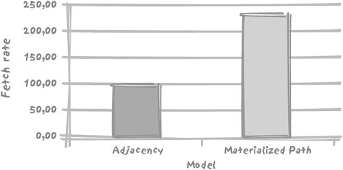 Simpler tree implementation sometimes performs quite well when computing aggregates. 7.5.2. Propagation of Percentages Across Different LevelsMust we conclude that with a materialized path and a pinch of adjacency where available we can solve anything more or less elegantly and efficiently? Unfortunately not, and our last example will really demonstrate the limits of some SQL implementations when it comes to handling trees. For this case, let's take a totally different example, and we will assume that we are in the business of potions, philters, and charms. Each of them is composed of a number of ingredientsand our recipes just list the ingredients and their percentage composition. Where is the hierarchy? Some of our recipes share a kind of "base philter" that appears as a kind of compound ingredient, as in Figure 7-5. Figure 7-5. Don't try this at home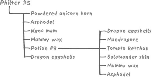 Our aim is, in order to satisfy current regulations, to display on the package of Philter #5 the names and proportions of all the basic ingredients. First, let's consider how we can model such a hierarchy. In such a case, a materialized path would be rather inappropriate. Contrarily to fighting units that have a single, well-defined place in the army hierarchy, any ingredient, including compound ones such as Potion #9, can contribute to many preparations. A path cannot be an attribute of an ingredient. If we decide to "flatten" compositions and create a new table to associate a materialized path to each basic ingredient in a composition, any change brought to Potion #9 would have to ripple through potentially hundreds of formulae, with the unacceptable risk in this line of business of one change going wrong. The most natural way to represent such a structure is therefore to say that our philter contains so much of powdered unicorn horn, so much of asphodel, and so much of Potion #9 and so forth, and to include the composition of Potion #9. Figure 7-6 illustrates one way we can model our database. We have a generic components table with two subtypes, recipes and basic_ingredients, and a composition table storing the quantity of a component (a recipe or a basic ingredient) that appears in each recipe. Figure 7-6. The model for recipes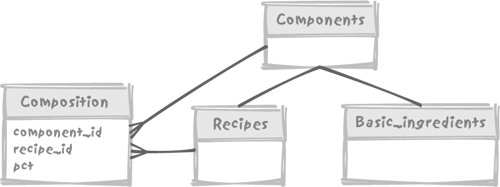 However, Figure 7-6's design is precisely where an approach such as connect by becomes especially clunky. Because of the procedural nature of the connect by operator, we can include only two levels, which could be enough for the case of Figure 7-5, but not in a general case. What do I mean by including two levels? With connect by we have the visibility of two levels at once, the current level and the parent level, with the possible exception of the root level. For instance: SQL> select connect_by_root recipe_id root_recipe, 2 recipe_id, 3 prior pct, 4 pct 5 component_id 6 from composition 7 connect by recipe_id = prior component_id 8 / ROOT_RECIPE RECIPE_ID PRIORPCT PCT COMPONENT_ID ----------- ---------- ---------- ------------ ------------ 14 14 5 3 14 14 20 7 14 14 15 8 14 14 30 9 14 14 20 10 14 14 10 2 15 15 30 14 15 14 30 5 3 15 14 30 20 7 15 14 30 15 8 15 14 30 30 9 ... In this example, root_recipe refers to the root of the tree. We can handle simultaneously the percentage of the current row and the percentage of the prior row, in tree-walking order, but we have no easy way to sum up, or in this precise case, to multiply values across a hierarchy, from top to bottom. The requirement for propagating percentages across levels is, however, a case where a recursive with statement is particularly useful. Why? Remember that when we tried to display the underlings of General Vandamme we had to compute the level to know how deep we were in the tree, carrying the result from level to level across our walk. That approach might have seemed cumbersome then. But that same approach is what will now allow us to pull off an important trick. The great weakness of connect by is that at one given point in time you can only know two generations: the current row (the child) and its parent. If we have only two levels, if Potion #9 contains 15% of Mandragore and Philter #5 contains 30% of Potion #9, by accessing simultaneously the child (Potion #9) and the parent (Philter #5) we can easily say that we actually have 15% of 30%in other words, 4.5% of Mandragore in Philter #5. But what if we have more than two levels? We may find a way to compute how much of each individual ingredient is contained in the final products with procedures, either in the program that accesses the database, or by invoking user-defined functions to store temporary results. But we have no way to make such a computation through plain SQL. "What percentage of each ingredient does a formula contain?" is a complicated question. The recursive with makes answering it a breeze. Instead of computing the current level as being the parent level plus 1, all we have to do is compute the actual percentage as being the current percentage (how much Mandragore we have in Potion #9) multiplied by the parent percentage (how much Potion #9 we have in Philter #5). If we assume that the names of the components are held in the components table, we can write our recursive query as follows: with recursive_composition(actual_pct, component_id) as (select a.pct, a.component_id from composition a, components b where b.component_id = a.recipe_id and b.component_name = 'Philter #5' union all select parent.pct * child.pct, child.component_id from recursive_composition parent, composition child where child.recipe_id = parent.component_id) Let's say that the components table has a component_type column that contains I for a basic ingredient and R for a recipe. All we have to do in our final query is filter (with an f ) recipes out, and, since the same basic ingredient can appear at various different levels in the hierarchy, aggregate per ingredient: select x.component_name, sum(y.actual_pct) from recursive_composition y, components x where x.component_id = y.component_id and x.component_type = 'I' group by x.component_name As it happens, even if the adjacency model looks like a fairly natural way to represent hierarchies, its two implementations are in no way equivalent, but rather complementary. While connect by may superficially look easier (once you have understood where prior goes) and is convenient for displaying nicely indented hierarchies, the somewhat tougher recursive with allows you to process much more complex questions relatively easilyand those complex questions are the type more likely to be encountered in real life. You only have to check the small print on a cereal box or a toothpaste tube to notice some similarities with the previous example of composition analysis. In all other cases, including that of a DBMS that implements a connect by, our only hope of generating the result from a "single SQL statement" is by writing a user-defined function, which has to be recursive if the DBMS cannot walk the tree. A more complex tree walking syntax may make a more complex question easier to answer in pure SQL. While the methods described in this chapter can give reasonably satisfactory results against very small amounts of data, queries using the same techniques against very large volumes of data may execute "as slow as molasses." In such a case, you might consider a denormalization of the model and a trigger-based "flattening" of the data. Many, including myself, frown upon denormalization. However, I am not recommending that you consider denormalizing for the oft-cited inherent slowness of the relational model, so convenient for covering up incompetent programming, but because SQL still lacks a truly adequate, scaleable processing of tree structures. |
EAN: 2147483647
Pages: 143