Protecting Worksheets

In addition to password protection for your files, Excel offers several features that you can use to protect your work-workbooks, workbook structures, individual cells, graphic objects, charts, scenarios, windows, and more-from access or modification by others. You can also choose to allow specific editing actions on protected worksheets.

For information about additional security issues in Excel, see Chapter 4, "Security and Privacy."

By default, Excel locks (protects) all cells and charts, but the protection is unavailable until you click the Review tab on the Ribbon and click Protect Sheet to access the Protect Sheet dialog box, as shown in Figure 6-22. (You can also click the Format button on the Home tab and then click Protect Sheet.) The protection status you specify applies to the current worksheet only.

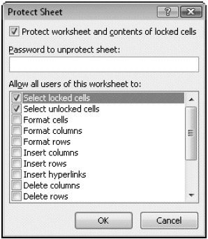
Figure 6-22: The Protect Sheet dialog box gives you pinpoint control over many common editing actions.

After protection is turned on, you cannot change a locked item. If you try to change a locked item, Excel displays an error message. As you can see in Figure 6-22, the Allow All Users Of This Worksheet To list contains a number of specific editorial actions you can allow on protected worksheets. In addition to the options visible in Figure 6-22, you can also allow users to sort, use Filter and PivotTable reports, and edit objects or scenarios.

Unlocking Individual Cells

If you click Protect Sheet without specifically unlocking individual cells, you'll lock every cell on the worksheet by default. Most of the time, however, you will not want to lock every cell. For example, you might want to protect the formulas and formatting but leave particular cells unlocked so you can type necessary data without unlocking the entire worksheet. Before you protect a worksheet, select the cells you want to keep unlocked, click Format on the Home tab, and click Lock Cell, as shown in Figure 6-23. Lock Cell is selected by default for all cells, so clicking it deselects it, unlocking the selected cells.

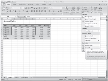
Figure 6-23: Click Format, Lock Cell to unlock specific cells for editing.

You can easily move between unprotected cells on a locked worksheet by pressing the Tab key.

One way to verify the locked status of a cell is to select it and look at the little padlock icon next to the Lock command. If the icon appears to be clicked already, it means that the selected cell is locked, which is the default state for all cells.

Note 

Keep in mind that Excel does not provide any on-screen indication of the protection status for individual cells. To distinguish unlocked cells from the protected cells, you might consider applying a specific format, such as cell color or borders.

Protecting the Workbook

You can prevent the alteration of a workbook's structure and lock the position of the workbook window. To do so, click the Review tab on the Ribbon, and click Protect Workbook, Protect Structure And Windows to display the dialog box shown in Figure 6-24.

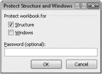
Figure 6-24: Use the Protect Structure And Windows dialog box to set the protection status for the entire workbook.

For more information, see "Protecting Workbooks" on page 176.

Allowing Password Access to Specific Cell Ranges

If you need to do more than protect workbooks or individual worksheets, use the Ribbon. Specifically, on the Review tab, in the Changes group, click Allow Users To Edit Ranges. Use the Allow Users To Edit Ranges dialog box, as shown in Figure 6-25, to provide editorial access to specific areas of a protected worksheet. You can even specify exactly who is allowed to do the editing.

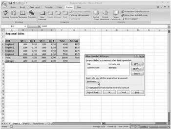
Figure 6-25: You can specify cells that can be edited, as well as the individuals who are allowed to edit them, by using the Allow Users To Edit Ranges dialog box.

When you click New in the Allow Users To Edit Ranges dialog box to add a cell range to the list, the New Range dialog box appears, as shown in Figure 6-26. Type a title for the range of cells you want to allow users to edit. Type a cell range or range name in the Refers To Cells box, or click in the box and drag through the range you want to specify.

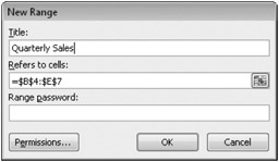
Figure 6-26: Specify ranges you want to allow users to edit using the New Range dialog box.

Selecting the Paste Permissions Information Into A New Workbook check box is a handy way to keep track of who and what you've specified in the Permissions list. Note that you can click the Protect Sheet button for quick access to the Protect Sheet dialog box shown in Figure 6-22. You can click the Permissions button to specify individuals who are allowed to edit each range. When you do so, a dialog box like the one in Figure 6-27 appears.

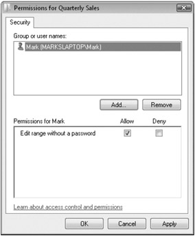
Figure 6-27: Set permissions for individual users by clicking Permissions in the Allow Users To Edit Ranges dialog box.

The Permissions dialog box lists all the users who are authorized to edit the worksheet, as well as whether they will need to use a password to do so. For each item in the Group Or User Names list, you can specify password permissions in the box; click Allow or Deny to restrict editing without a password. This lets you, in effect, employ two levels of restriction, since you are restricting editing access to specified users anyway, and you can force even those users to type a password if you want to do so.

Note 

You must specify a password in the New Range dialog box (shown in Figure 6-26) or in the identical Modify Range dialog box to turn on the permissions options that you set. If you don't specify a range password, anyone can edit the range.

You can add users and groups to the list in the Permissions dialog box by clicking Add and then clicking Advanced to display the full dialog box shown in Figure 6-28. Click Find Now to locate all the users and groups available to your system. However, if you are connected to a large network, this might take a long time, so you can use the Common Queries box to restrict your search. You can also use Object Types and Locations to restrict your search further. After you click Find Now, you can select items in the list at the bottom of the dialog box that you want to add. Press the Ctrl key to select multiple items. When you have located the users and groups you want to add, click OK.

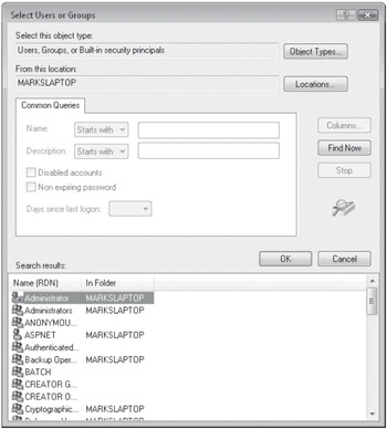
Figure 6-28: Click Add in the Permissions dialog box to add to your list of authorized users.

Note 

To add or change users on your computer, open User Accounts in Control Panel.

Remember, after all this, you still have to activate worksheet protection by clicking Protect Sheet on the Home tab or by clicking Protect Sheet in the Allow Users To Edit Ranges dialog box.

For information about setting file-level permissions, see "Controlling Document Access with Information Rights Management" on page 803. For information about Excel and networks, see "Sharing Workbooks on a Network" on page 790.

Hiding Cells and Worksheets

In a protected worksheet, if you applied the Hidden protection format to a cell that contains a formula, the formula remains hidden from view in the formula bar, even when you select that cell. To hide a selected cell or cells, click the Format button on the Home tab, and click Cells to display the Format Cells dialog box. Then click the Protection tab, and select the Hidden option. Formulas in hidden cells are still functional, of course; they are just hidden from view. In any case, the displayed result of the formula on the worksheet is still visible.

For information about hiding numbers, see "The Hidden Number Format" on page 315.

You can also hide rows and columns within a worksheet and even hide entire worksheets within a workbook. Any data or calculations in hidden rows, columns, or worksheets are still available through references; the cells or worksheets are hidden from view. To hide a worksheet, click the sheet tab of the worksheet you want to hide, and on the Home tab, click Format, Hide & Unhide, Hide Sheet, as shown in Figure 6-29. Unlike hiding cells, hiding rows, columns, or worksheets happens immediately. Afterward, you can click the corresponding Unhide command to restore the hidden item.

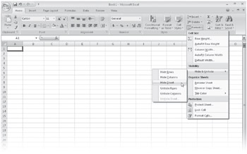
Figure 6-29: Use the Hide & Unhide commands to protect parts of your workbooks.

However, if you hide a worksheet and then click Protect Workbook on the Review tab, the Unhide command is no longer available, which helps keep the hidden worksheet even better protected.

For more information about workbook protection, see "Hiding and Protecting Workbooks" on page 175.

Using Passwords

When you click Protect Sheet, Protect Workbook, or Protect And Share Workbook on the Review tab, you can assign a password that must be used to disable the protection. You can use unique passwords for each worksheet or workbook you protect.

Caution 

Password protection in Excel is serious business. After you assign a password, you can't unprotect the worksheet or workbook without it. Don't forget your passwords! Remember, capitalization matters.