What Is a Vector?

 

Higher-Degree Polynomials

Consider, if you will, the selection of curves shown in Figure 1.2.

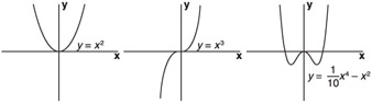
Figure 1.2: Higher-degree polynomials.

The last section talked quite a bit about slopes, but the curves in Figure 1.2 do not have a constant slope. In fact, the leftmost curve has a different slope at each and every point along the curve. At this point, life suddenly becomes more complicated. Figure 1.3 shows you why. Both pictures show a bullet moving along a path. In the left picture, the bullet is moving along a straight line. You can easily say that the direction of the bullet at any point along the path is the same as the slope of the line. In the right picture, the bullet follows a curved path. It is still true that the direction of the bullet matches the slope of the curve, but the direction changes.

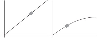
Figure 1.3: Bullets along different paths.

You can draw a curve without caring too much about the slope at any given point, but you can't correctly draw the bullet if you don't know how to find the slope at that point. This is where calculus comes in handy. If you aren't familiar with calculus, now might be a good time to jump ahead to Appendix A, "Derivative Calculus." I have included a short tutorial on differential calculus that will provide you with the basic tools you need to move forward.

You can find the slope at any point along the curve by finding the derivative of the curve at that point. For simple polynomials, this process is relatively easy because the functions are easy to differentiate. Once you know how to find the slope at any point, you can use derivatives to gain a better understanding of nearly any polynomial function.

As an example, let's say I tell you that the distance covered by a falling object is given by the following equation.

(1.5) Simple equation for the distance covered by a falling object. 

In fact, this equation is correct if you assume that the initial position and velocity are zero. From this, you can draw the graph in Figure 1.4.

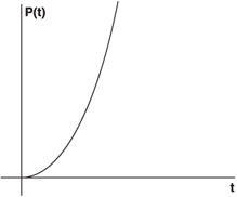
Figure 1.4: The distance covered by a falling object over time.

This graph shows that the object moved small distances at first, but large distances later. This would imply that the velocity grew over time. In fact, the velocity at any point in time is the slope of the position curve at that time. As outlined in Appendix A, you can find the slope using differential calculus. To find the velocity at time t, differentiate Equation 1.5 to get the following equation.

(1.6) The first derivative of Equation 1.5. 

Equation 1.6 describes how the position of an object changes as time changes. This is the speed of the object. Speed is how fast something changes with respect to time. It is also the first derivative of the distance.

Note 

Remember that speed and velocity are different. Speed is a simple scalar value. Velocity is a vector value. The distinction isn't terribly important in this context, but I don't want to lead you astray.

If you graph Equation 1.6, you'll get the graph shown in Figure 1.5.

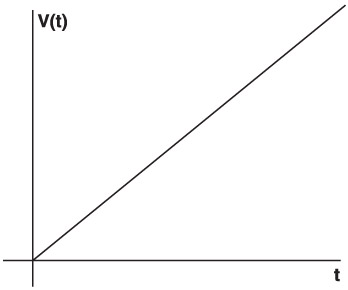
Figure 1.5: The speed of a falling object over time.

This is the graph of the values of the slope. In Figure 1.4, you could see that the slope was increasing. Figure 1.5 shows that the slope (and therefore the speed) is increasing linearly.

Now, go one step further and differentiate this. The derivative of speed is acceleration. Acceleration is the measure of how the speed changes over time. In this case, the derivative is a constant, as shown in Equation 1.7. Figure 1.6 shows the very simple resulting graph.

Figure 1.6: The acceleration of a falling object over time.

(1.7) The second derivative of Equation 1.5. 

Figure 1.6 shows that the acceleration of the object was constant throughout time. This is true for falling objects. Gravity remains effectively constant unless you are talking about measuring very small changes and falling very long distances. So, you can see that the derivatives do accurately reflect what is actually happening.

Figure 1.7 condenses these three steps into three graphs. In this case, the equation for the distance is a polynomial of a higher degree. You can see that the acceleration is not constant. Instead, it increases linearly over time. These graphs could be showing the behavior of a car where the driver is slowly increasing pressure on the gas pedal over time.

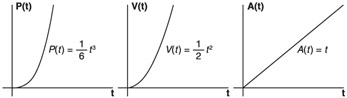
Figure 1.7: The distance, speed, and acceleration of a moving object.

In most cases, you will not need to derive these characteristics because you will know them already. The purpose of the preceding examples was to get you thinking about how curves work and the meaning behind the features of both the graphs and the equations. As the next section will show, you will have an easier time understanding and implementing the behavior of an object if you understand exactly how a curve is affecting that object.