Monitoring Query Performance

Before you think about taking some action to make a query faster, such as adding an index or denormalizing, you should understand how a query is currently being processed. You should also get some baseline performance measurements so you can compare behavior both before and after making your changes. SQL Server provides these tools (SET options) for monitoring queries:

• STATISTICS IO
• STATISTICS TIME
• SHOWPLAN

You enable any of these SET options before you run a query, and they will produce additional output. Typically, you run your query with these options set in a tool such as SQL Query Analyzer. When you're satisfied with your query, you can cut and paste it into your application or into the script file that creates your stored procedures. If you use the SET commands to turn these options on, they apply only to the current connection. SQL Query Analyzer provides check boxes for turning any or all of these options on or off for all connections.

STATISTICS IO

Don't let the term statistics fool you. STATISTICS IO doesn't have anything to do with the statistics used for storing histograms and density information in sysindexes. This option provides statistics on how much work SQL Server did to process your query. When this option is set to ON, you get a separate line of output for each query in a batch that accesses any data objects. (You don't get any output for statements that don't access data, such as PRINT, SELECT the value of a variable, or call a system function.) The output from SET STATISTICS IO ON includes the values Logical Reads, Physical Reads, Read Ahead Reads, and Scan Count.

Logical Reads

This value indicates the total number of page accesses needed to process the query. Every page is read from the data cache, whether or not it was necessary to bring that page from disk into the cache for any given read. This value is always at least as large and usually larger than the value for Physical Reads. The same page can be read many times (such as when a query is driven from an index), so the count of Logical Reads for a table can be greater than the number of pages in a table.

Physical Reads

This value indicates the number of pages that were read from disk; it is always less than or equal to the value of Logical Reads. The value of the Buffer Cache Hit Ratio, as displayed by System Monitor, is computed from the Logical Reads and Physical Reads values as follows:

 Cache-Hit Ratio = (Logical Reads _ Physical Reads) / Logical Reads 

Remember that the value for Physical Reads can vary greatly and decreases substantially with the second and subsequent execution because the cache is loaded by the first execution. The value is also affected by other SQL Server activity and can appear low if the page was preloaded by read ahead activity. For this reason, you probably won't find it useful to do a lot of analysis of physical I/O on a per-query basis. When you're looking at individual queries, the Logical Reads value is usually more interesting because the information is consistent. Physical I/O and achieving a good cache-hit ratio is crucial, but they are more interesting at the all-server level. Pay close attention to Logical Reads for each important query, and pay close attention to physical I/O and the cache-hit ratio for the server as a whole.

STATISTICS IO acts on a per-table, per-query basis. You might want to see the physical_io column in sysprocesses corresponding to the specific connection. This column shows the cumulative count of synchronous I/O that has occurred during the spid's existence, regardless of the table. It even includes any Read Ahead Reads that were made by that connection.

Read Ahead Reads

The Read Ahead Reads value indicates the number of pages that were read into cache using the read ahead mechanism while the query was processed. These pages are not necessarily used by the query. If a page is ultimately needed, a logical read is counted but a physical read is not. A high value means that the value for Physical Reads is probably lower and the cache-hit ratio is probably higher than if a read ahead was not done. In a situation like this, you shouldn't infer from a high cache-hit ratio that your system can't benefit from additional memory. The high ratio might come from the read ahead mechanism bringing much of the needed data into cache. That's a good thing, but it might be better if the data simply remains in cache from previous use. You might achieve the same or a higher cache-hit ratio without requiring the Read Ahead Reads.

You can think of read ahead as simply an optimistic form of physical I/O. In full or partial table scans, the table's IAMs are consulted to determine which extents belong to the object. The extents are read with a single 64 KB scatter read, and because of the way that the IAMs are organized, they are read in disk order. If the table is spread across multiple files in a file group, the read ahead attempts to keep at least eight of the files busy instead of sequentially processing the files. Read Ahead Reads are asynchronously requested by the thread that is running the query; because they are asynchronous, the scan doesn't block while waiting for them to complete. It blocks only when it actually tries to scan a page that it thinks has been brought into cache and the read hasn't finished yet. In this way, the read ahead neither gets too ambitious (reading too far ahead of the scan) nor too far behind.

Scan Count

The Scan Count value indicates the number of times that the corresponding table was accessed. Outer tables of a nested loop join have a Scan Count of 1. For inner tables, the Scan Count might be the number of times "through the loop" that the table was accessed. The number of Logical Reads is determined by the sum of the Scan Count times the number of pages accessed on each scan. However, even for nested loop joins, the Scan Count for the inner table might show up as 1. SQL Server might copy the needed rows from the inner table into a worktable in cache and use this worktable to access the actual data rows. When this step is used in the plan, there is often no indication of it in the STATISTICS IO output. You must use the output from STATISTIC TIME, as well as information about the actual processing plan used, to determine the actual work involved in executing a query. Hash joins and merge joins usually show the Scan Count as 1 for both tables involved in the join, but these types of joins can involve substantially more memory. You can inspect the memusage value in sysprocesses while the query is being executed, but unlike the physical_io value, this is not a cumulative counter and is valid only for the currently running query. Once a query finishes, there is no way to see how much memory it used.

Troubleshooting Example Using STATISTICS IO

The following situation is based on a real problem I encountered when doing a simple SELECT * from a table with only a few thousand rows. The amount of time this simple SELECT took seemed to be out of proportion to the size of the table. We can create a similar situation here by making a copy of the orders table in the Northwind database and adding a new column to it with a default value of 2000-byte character field.

 SELECT * INTO neworders FROM orders GO ALTER TABLE neworders ADD full_details CHAR(2000) NOT NULL DEFAULT 'full details' 

We can gather some information about this table with the following command:

 EXEC sp_spaceused neworders, true 

The results will tell us that there are 830 rows in the table, 3240 KB for data, which equates to 405 data pages. That doesn't seem completely unreasonable, so we can try selecting all the rows after enabling STATISTICS IO:

 SET STATISTICS IO ON GO SELECT * FROM neworders 

The results now show that SQL Server had to perform 1945 logical reads for only 405 data pages. There is no possibility that a nonclustered index is being used inappropriately, because I just created this table, and there are no indexes at all on it. So where are all the reads coming from?

Recall that if a row is increased in size so that it no longer fits on the original page, it will be moved to a new page, and SQL Server will create a forwarding pointer to the new location from the old location. In Chapter 9, I told you about two ways to find out how many forwarding pointers were in a table: we could use the undocumented trace flag 2509, or we could run DBCC SHOWCONTIG with the TABLERESULTS options. Here, I'll use the trace flag:

 DBCC TRACEON (2509) GO DBCC CHECKTABLE (neworders) RESULTS: DBCC execution completed. If DBCC printed error messages, contact your system administrator. DBCC results for 'neworders'. There are 830 rows in 405 pages for object 'neworders'. Forwarded Record count = 770 

If you play around with the numbers a bit, you might realize that 2*770 + 405 equals 1945, the number of reads we ended up performing with the table scan. What I realized was happening was that when scanning a table, SQL Server will read every page (there are 405 of them), and each time a forwarding pointer is encountered, SQL Server will jump ahead to that page to read the row and then jump back to the page where the pointer was and read the original page again. So for each forwarding pointer, there are two additional logical reads. SQL Server is doing a lot of work here for a simple table scan.

The "fix" to this problem is to regularly check the number of forwarding pointers, especially if a table has variable-length fields and is frequently updated. If you notice a high number of forwarding pointers, you can rebuild the table by creating a clustered index. If for some reason I don't want to keep the clustered index, I can drop it. But the act of creating the clustered index will reorganize the table.

 SET STATISTICS IO OFF GO CREATE CLUSTERED INDEX orderID_cl ON neworders(orderID) GO DROP INDEX neworders.orderID_cl GO EXEC sp_spaceused neworders, true SET STATISTICS IO ON GO SELECT ROWS = count(*) FROM neworders RESULTS: name rows reserved data index_size unused --------------- -------- ---------- --------- ------------- ------ neworders 830 2248 KB 2216 KB 8 KB 24 KB ROWS ----------- 830 (1 row(s) affected) Table 'neworders'. Scan count 1, logical reads 277, physical reads 13, read-ahead reads 278. 

This output shows us that not only did the building of the clustered index reduce the number of pages in the table, from 405 to 277, but the cost to read the table is now the same as the number of pages in the table.

STATISTICS TIME

The output of SET STATISTICS TIME ON is pretty self-explanatory. It shows the elapsed and CPU time required to process the query. In this context, it means the time not spent waiting for resources such as locks or reads to complete. The times are separated into two components: the time required to parse and compile the query, and the time required to execute the query. For some of your testing, you might find it just as useful to look at the system time with getdate before and after a query if all you need to measure is elapsed time. However, if you want to compare elapsed vs. actual CPU time or if you're interested in how long compilation and optimization took, you must use STATISTICS TIME.

In many cases, you'll notice that the output includes two sets of data for parse and compile time. This happens when the plan is being added to syscacheobjects for possible reuse. The first line is the actual parse and compile before placing the plan in cache, and the second line appears when SQL Server is retrieving the plan from cache. Subsequent executions will still show the same two lines, but if the plan is actually being reused, the parse and compile time for both lines will be 0.

Showplan

In SQL Server 2000, there is not just a single option for examining the execution plan for a query. You can choose to see the plan in a text format, with or without additional performance estimates, or you can see a graphical representation of the processing plan. In Chapter 15, I gave you a sneak preview of the graphical showplan. Now I'll go into more detail.

The output of any of the showplan options shows some basic information about how the query will be processed. The output will tell you, for each table in the query, whether indexes are being used or whether a table scan is necessary. It will also tell you the order that all the different operations of the plan are to be carried out. Reading showplan output is as much an art as it is a science, but for the most part it just takes a lot of practice to get really comfortable with its interpretation. I hope that the examples in this section will be enough to give you a good start.

SHOWPLAN_TEXT and SHOWPLAN_ALL

The two SET options SHOWPLAN_TEXT and SHOWPLAN_ALL let you see the estimated query plan without actually executing the query. Both options also automatically enable the SET NOEXEC option, so you don't see any results from your query—you see only the way that SQL Server has determined is the best method for processing the query. Turning NOEXEC ON can be a good thing while tuning a query. For example, if you have a query that takes 20 minutes to execute, you might try to create an index that will allow it to run faster. However, immediately after creating a new index, you might just want to know whether the query optimizer will even choose to use that index. If you were actually executing the query every time you looked at its plan, it would take you 20 minutes for every tuning attempt. Setting NOEXEC ON along with the showplan option will allow you to see the plan without actually executing all the statements.

WARNING

---

Since turning on SHOWPLAN_TEXT or SHOWPLAN_ALL implies that NOEXEC is also on, you must set the SHOWPLAN option to OFF before you do anything else. For example, you must set SHOWPLAN_TEXT to OFF before setting SHOWPLAN_ALL to ON.

SHOWPLAN_TEXT shows you all the steps involved in processing the query, including the type of join used, the order of table accesses, and which index or indexes are used for each table. Any internal sorts are also shown. Here's an example of a simple two-table join from the Northwind database:

 SET SHOWPLAN_TEXT ON GO SELECT ProductName, Products.ProductId FROM [Order Details] JOIN Products ON [Order Details].ProductID = Products.ProductId WHERE Products.UnitPrice > 10 GO OUTPUT: StmtText ---------------------------------------------------------------------- |--Nested Loops(Inner Join, OUTER REFERENCES:([Products].[ProductID])) |--Clustered Index Scan (OBJECT:([Northwind].[dbo].[Products].[PK_Products]), WHERE:([Products].[UnitPrice]>10.00)) |--Index Seek (OBJECT:([Northwind].[dbo].[Order Details].[ProductID]), SEEK:([Order Details].[ProductID]=[Products].[ProductID]) ORDERED FORWARD) 

The output tells us that the query plan is performing an inner join on the two tables. Inner Join is the logical operator, as requested in the query submitted. The way that this join is actually carried out is the physical operator; in this case, the query optimizer chose to use nested loops. The outer table in the join is the Products table, and a Clustered Index Scan is the physical operator. In this case, there is no separate logical operator—the logical operator and the physical operator are the same. Remember that since a clustered index contains all the table data, scanning the clustered index is equivalent to scanning the whole table. The inner table is the Order Details table, which has a nonclustered index on the ProductID column. The physical operator used is Index Seek. The Object reference after the Index Seek operator shows us the full name of the index used: :([Northwind].[dbo].[Order Details].[ProductID]. In this case, it is a bit confusing because the name of the index is the same as the name of the join column. For this reason, I recommend not giving indexes the same names as the columns they will access.

SHOWPLAN_ALL provides this information plus estimates of the number of rows that are expected to meet the queries' search criteria, the estimated size of the result rows, the estimated CPU time, and the total cost estimate that was used internally when comparing this plan to other possible plans. I won't show you the output from SHOWPLAN_ALL because it's too wide to fit nicely on a page of this book. But the information returned is the same as the information you'll be shown with the graphical showplan, and I'll show you a few more examples of graphical plans in this chapter.

When using showplan to tune a query, you typically add one or more indexes that you think might help speed up a query and then you use one of these showplan options to see whether any of your new indexes were actually used. If showplan indicates that a new index is being used, you should then actually execute the query to make sure that the performance is improved. If an index is not going to be used or is not useful in terms of performance improvement, and you're not adding it to maintain a Primary Key or Unique constraint, you might as well not add it. If an index is not useful for queries, the index is just overhead in terms of space and maintenance time. After you add indexes, be sure to monitor their effect on your updates because indexes can add overhead to data modification (inserts, deletes, and updates).

If a change to indexing alone is not the answer, you should look at other possible solutions, such as using an index hint or changing the general approach to the query. In Chapter 10, you saw that several different approaches can be useful to some queries—ranging from the use of somewhat tricky SQL to the use of temporary tables and cursors. If these approaches also fail to provide acceptable performance, you should consider changes to the database design using the denormalization techniques discussed earlier.

Graphical Showplan

You can request a graphical representation of a query's estimated execution plan in SQL Query Analyzer either by using the Display Estimated Execution Plan toolbar button immediately to the right of the database drop-down list or by choosing Display Estimated Execution Plan from the Query menu. Like the SET options SHOWPLAN_TEXT and SHOWPLAN_ALL, by default your query is not executed when you choose to display the graphical showplan output. The graphical representation contains all the information available through SHOWPLAN_ALL, but not all of it is visible at once. You can, however, move your cursor over any of the icons in the graphical plan to see the additional performance estimates.

Figure 16-3 shows the graphical query plan for the same query I used in the previous section, and I've put my cursor over the icon for the nested loop join so you can see the information box. When reading the graphical showplan, you need to read from right to left. When you look at the plan for a JOIN, the table listed on the top is the first one processed. For a LOOP join, the top table is the outer table, and for a HASH join, the top table is the build table. The figure shows that the Products table is accessed first as the outer table in a Nested Loop join, and the other table would be the inner table. You can't see the other table in the figure because the information box is covering it up. The final step in the plan, shown on the far left, is to actually SELECT the qualifying rows and return them to the client.

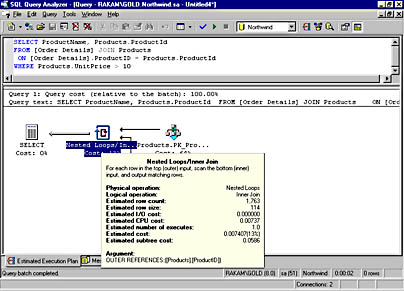
Figure 16-3. A graphical showplan showing a nested loop join operation.

Table 16-1, taken from SQL Server Books Online, describes the meaning of each of the output values that you can see in the details box for the Nested Loops icon. Some of these values, for example StmtId, NodeId, and Parent, do not show up in the graphical representation—only in the SHOWPLAN_ALL output.

Table 16-1. Values available in the showplan output.

Column	What It Contains
StmtText	The text of the Transact-SQL statement.
StmtId	The number of the statement in the current batch.
NodeId	The ID of the node in the current query.
Parent	The node ID of the parent step.
PhysicalOp	The physical implementation algorithm for the node.
LogicalOp	The relational algebraic operator that this node represents.
Argument	Supplemental information about the operation being performed. The contents of this column depend on the physical operator.
DefinedValues	A comma-separated list of values introduced by this operator. These values can be computed expressions that were present in the current query (for example, in the SELECT list or WHERE clause) or internal values introduced by the query processor in order to process this query. These defined values can then be referenced elsewhere within this query.
EstimateRows	The estimated number of rows output by this operator.
EstimateIO	The estimated I/O cost for this operator.
EstimateCPU	The estimated CPU cost for this operator.
AvgRowSize	The estimated average row size (in bytes) of the row being passed through this operator.
TotalSubtreeCost	The estimated (cumulative) cost of this operation and all child operations.
OutputList	A comma-separated list of columns being projected by the current operation.
Warnings	A comma-separated list of warning messages relating to the current operation.
Type	The node type. For the parent node of each query, this is the Transact-SQL statement type (for example, SELECT, INSERT, EXECUTE, and so on). For subnodes representing execution plans, the type is PLAN_ROW.
Parallel	0 = Operator is not running in parallel. 1 = Operator is running in parallel.
EstimateExecutions	The estimated number of times this operator will be executed while running the current query.

Let's look at a slightly more complex query plan for this query based on a four-table join and a GROUP BY with aggregation.

 USE Northwind SELECT e.LastName, p.ProductName, sum(d.Quantity * d.UnitPrice) FROM [Order Details] d JOIN Orders o ON o.OrderID = d.OrderID JOIN Products p ON d.ProductID = p.ProductID JOIN Employees e ON e.EmployeeID = o.EmployeeID GROUP BY e.LastName, p.ProductName 

You can see most of the graphical plan in Figure 16-4. Because there are four tables, the plan shows three join operators. You need to read the plan from right to left, and you can see that the Employees and Orders tables are joined with a Nested Loops join, and then the result of that first join is joined with the Order Details table, again using Nested Loops. Finally, the result of the second join is joined with the Products table using hashing. Note that the order that the joins are processed in the plan is not at all the same order used when writing the query. The query optimizer attempts to find the best plan regardless of how the query was actually submitted. The final step is to do the grouping and aggregation, and the graphical plan shows us that this was done using hashing.

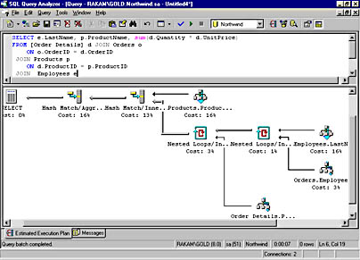
Figure 16-4. A graphical showplan for a four-table join with GROUP BY aggregation.

WARNING

---

In order to generate the graphical showplan, SQL Server must make sure that both SHOWPLAN_TEXT and SHOWPLAN_ALL are in the OFF state so that the NOEXEC option is also OFF. If you've been tuning queries using the SHOWPLAN_TEXT option and you then decide to look at a graphical showplan, the NOEXEC option will be left in the OFF state after you view the graphical plan. If you then try to go back to looking at SHOWPLAN_TEXT, you'll find that it has been turned off, and any queries you run will actually be executed.

Troubleshooting with Showplan

One of the first things to look for in your showplan output is whether there are any warning messages. Warning messages might include the string "NO STATS:()" with a list of columns. This warning message means that the query optimizer attempted to make a decision based on the statistics for this column but that no statistics were available. Consequently, the query optimizer had to make a guess, which might have resulted in the selection of an inefficient query plan. Warnings can also include the string MISSING JOIN PREDICATE, which means that a join is taking place without a join predicate to connect the tables. Accidentally dropping a join predicate might result in a query that takes much longer to run than expected and returns a huge result set. If you see this warning, you should verify that the absence of a join predicate is what you wanted, as in the case of a CROSS JOIN.

Another area where SHOWPLAN can be useful is for determining why an index wasn't chosen. You can look at the estimated row counts for the various search arguments. Remember that a nonclustered index will mainly be useful if only a very small percentage of rows in the table will qualify; if the showplan output shows hundreds of rows meeting the condition, that can be a good indication of why a nonclustered index was not chosen. However, if the row estimate is very different from what you know it to actually be, you can look in two places for the reason. First make sure statistics are updated or that you haven't turned off the option to automatically update statistics on indexes. Second, make sure your WHERE clause actually contains a SARG and that you haven't invalidated the use of the index by applying a function or other operation to the indexed column. You saw an example of this problem in Chapter 15, and the plan was shown in Figure 15-4.

Another thing to remember from Chapter 15 is that there is no guarantee that the query optimizer will find the absolute fastest plan. It will search until it finds a good plan; there might actually be a faster plan, but the query optimizer might take twice as long to find it. The query optimizer decides to stop searching when it finds a "good enough" plan because the added cost of continued searching might offset whatever slight savings in execution time you'd get with a faster plan.

Here's an example. We'll build a table with big rows, each of which has a char(7000), so it needs one page per row. We'll then populate this table with 1000 rows of data and build three indexes:

 CREATE TABLE emps( empid int not null identity(1,1), fname varchar(10) not null, lname varchar(10) not null, hiredate datetime not null, salary money not null, resume char(7000) not null) GO -- populate with 1000 rows, each of which will fill a page SET NOCOUNT ON DECLARE @i AS int SET @i = 1 WHILE @i <= 1000 BEGIN INSERT INTO emps VALUES('fname' + cast(@i AS varchar(5)), 'lname' + cast(@i AS varchar(5)), getdate() - @i, 1000.00 + @i % 50, 'resume' + cast(@i AS varchar(5))) SET @i = @i + 1 END GO CREATE CLUSTERED INDEX idx_ci_empid ON [dbo].[emps] ([empid]) CREATE NONCLUSTERED INDEX idx_nci_lname ON [dbo].[emps] ([lname]) CREATE NONCLUSTERED INDEX idx_nci_fname ON [dbo].[emps] ([fname]) GO 

The query we'll execute will only access the fname and lname columns. As you've seen, SQL Server uses the index intersection technique to use two nonclustered indexes to determine the qualifying rows and join the results from the two indexes together. However, the optimizer decided not to use that plan in this case:

 SELECT fname, lname FROM emps 

The plan shows a clustered index scan, which means that the entire table is examined. The number of logical reads is about equal to the number of pages in the table (1002). However, if we apply a SARG that actually includes the whole table, we'll find that the query optimizer will use the index intersection technique. Here's the query:

 SELECT fname, lname FROM emps WHERE fname BETWEEN 'fname' and 'fname9999' 

Figure 16-5 shows the query plan using an index seek on the nonclustered index on fname and an index scan on the nonclustered index on lname, and then using a hash join to combine the result sets of the two index operations. If we turn on STATISTICS IO, the logical reads are reported to be only 8 pages. It might seem as if the difference between 8 logical reads and 1000 logical reads is a lot, but in the grand scheme of things, it really isn't all that much. Reading 1000 pages is still a very fast operation, and the query optimizer decided not to search further. It will only consider the index intersection case if it already is doing index seek operations, and with no SARGs in the query, index seek is not an option.

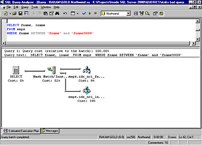
Figure 16-5. A graphical showplan for an index intersection when index seek operations are used.

However, if the table has more than 1000 rows, the situation changes. If we drop the emps table and re-create it with 10,000 rows instead of 1000, the cost of doing the simple clustered index scan becomes 10,000 logical reads. In this case, that is deemed too expensive, so the query optimizer will keep searching for a better plan. With 10,000 rows in the emps table, the index intersection technique is evaluated and found to be faster. In fact, it will take only about 60 logical reads, which is a big improvement over 10,000.

Logical and Physical Operators

The logical and physical operators describe how a query or update was executed. The physical operators describe the physical implementation algorithm used to process a statement—for example, scanning a clustered index or performing a merge join. Each step in the execution of a query involves a physical operator. The logical operators describe the relational algebraic operation used to process a statement—for example, performing an aggregation or an inner join. Not all steps used to process a query or update involve logical operations.

Logical operators map pretty closely to what is contained in the query itself. As you've seen, you might have an inner join for the logical operator. The physical operator is then how the query optimizer decided to process that join—for example as a nested loop join, a hash join, or a merge join. Aggregation is a logical operator because the query actually specifies a GROUP BY with an aggregate and the corresponding physical operator, as chosen by the query optimizer, could be stream aggregate (if the grouping is done by sorting) or hash match (if the grouping is done by hashing).

You might see some types of joins that you don't recognize. I've already talked about inner joins; left, right and full outer joins; and cross joins. You might also see the following logical operators: Left Semi Join, Right Semi Join, Left Anti Semi Join, and Right Anti Semi Join. These sound mysterious, but they're really not. Normally, in a join, you're interested in columns from both tables. But if you use a subquery with an EXISTS or IN predicate, you're saying that you're not interested in retrieving data from the inner table and you're using it only for lookup purposes. So instead of needing data from both tables, you need data from only one of the tables, and this is a Semi Join. If you're looking for data from the outer table that doesn't exist in the inner table, it becomes an Anti Semi Join.

Here's an example in the pubs database that retrieves all the names of publishers that don't have corresponding pub_id values in the titles table—in other words, publishers who haven't published any books:

 USE pubs GO SELECT pub_name FROM publishers WHERE pub_id NOT IN (SELECT pub_id FROM titles) 

Here's the SHOWPLAN_TEXT output that the query generates. You can see the Left Anti Semi Join operator.

 StmtText ----------------------------------------------------------------------- |--Nested Loops(Left Anti Semi Join, WHERE:([titles].[pub_id]=NULL OR [publishers].[pub_id]=[titles].[pub_id])) |--Clustered Index Scan(OBJECT:([pubs].[dbo].[publishers].[UPKCL_pubind])) |--Clustered Index Scan(OBJECT:([pubs].[dbo].[titles].[UPKCL_titleidind])) 

Displaying the Actual Plan

All of the showplan options discussed so far show the estimated query plan. As long as the query is not actually being executed, you can only see an estimate. As you saw in Chapter 15, conditions such as memory resources might change before you actually run the query, so the estimated plan might not be the actual plan. If you need to see the actual plan at the time the query is executed, you have three options:

• Choose Show Execution Plan from the Query menu in SQL Query Analyzer. Unlike the Display Estimated Execution Plan option, this one acts like a toggle. Once you select it, it stays selected until you deselect it. You'll see two tabs of results for every query you run until you deselect Show Execution Plan. The first tab shows the actual query output, and the second shows the graphical showplan.
• Set STATISTICS PROFILE to ON. This option gives you the query results followed by the STATISTICS_ALL output in the same results pane.
• Set up a trace in SQL Profiler to capture the Execution Plan events. This displays from the same information as SHOWPLAN_TEXT in the trace output for every query that is executed. We'll look at tracing in more detail in Chapter 17.

Other SQL Query Analyzer Tools

In SQL Server 2000, SQL Query Analyzer provides other troubleshooting information besides SHOWPLAN and statistical output. Two additional options on the Query menu act as toggles to provide more information for every query that you run: Show Server Trace and Show Client Statistics. Each of these options, when enabled, adds another tab to the results window. The Server Trace output gives information similar to what you might see when you use SQL Profiler, which I'll discuss in Chapter 17. The Client Statistics output can give you a set of very useful data that indicates how much work the client had to do to submit this query and retrieve the results from SQL Server. It includes information that can also be returned by other means, such as the time spent and the number of rows affected, and it can also give additional information such as the number of bytes sent and received across the network.

Let's look at one of the Northwind queries I ran earlier and see what the client statistics look like when I execute it. Here's the query again:

 SELECT e.LastName, p.ProductName, sum(d.Quantity * d.UnitPrice) FROM [Order Details] d JOIN Orders o ON o.OrderID = d.OrderID JOIN Products p ON d.ProductID = p.ProductID JOIN Employees e ON e.EmployeeID = o.EmployeeID GROUP BY e.LastName, p.ProductName 

Here's the information that Client Statistics returned:

Counter	Value	Average
Application Profile Statistics:
Timer resolution (milliseconds)	0	0
Number of INSERT, UPDATE, DELETE statements	0	0
Rows effected by INSERT, UPDATE, DELETE statements	0	0
Number of SELECT statements	1	1
Rows effected by SELECT statements	588	588
Number of user transactions	1	1
Average fetch time	0	0
Cumulative fetch time	0	0
Number of fetches	0	0
Number of open statement handles	0	0
Max number of opened statement handles	0	0
Cumulative number of statement handles	0	0
Network Statistics:
Number of server roundtrips	1	1
Number of TDS packets sent	1	1
Number of TDS packets received	9	9
Number of bytes sent	552	552
Number of bytes received	35,921	35,921
Time Statistics:
Cumulative client processing time	223	223
Cumulative wait time on server replies	3	3

The number in the Value column pertains only to the most recently run batch. The number in the Average column is a cumulative average since you started collecting client statistics for this session. If you turn off the option to collect client statistics and then turn it on again, the numbers in the Average column will be reset.

There are a few other interesting features in SQL Query Analyzer that you should know about. I don't want to go into a lot of detail because this isn't a book about pointing and clicking your way through the tools and most of these tools aren't directly related to tuning your queries. But the more fluent you are in your use of this tool, the more you can use it to maximum benefit when you perform troubleshooting and tuning operations. This is not a complete list of all the capabilities of SQL Query Analyzer. I suggest you read SQL Server Books Online thoroughly and spend some time just exploring this tool even if you already think you know how to use it. I'll bet you'll discover something new. For a start, take a look at these options:

Object Browser The Object Browser is a tree-based tool window for navigating through the database objects of a selected SQL Server. Besides navigation, the Object Browser offers object scripting and procedure execution. To limit the overhead of using the Object Browser, only one server can be active at a time. The drop-down list box at the top of the Object Browser presents a distinct list of server names to which you can connect, and this means that you must have a connection already open to a server before you can use the Object Browser. The Object Browser has no explicit connect logic: it piggybacks on the existing query window connection's information.

Changing Fonts You can right-click in almost any window and choose the option to change your font. Alternatively, you can choose Options from the Tools menu and go to the Fonts tab, where you can set the font of any type of window.

Quick Edit From the Edit menu, you can choose to set or clear bookmarks, go to a specific line in the query window, change text to uppercase or lowercase, indent or unindent a block of code, or comment out a whole block of code.

Shortcut Keys You can configure the Ctrl+1 through Ctrl+0 and Alt+F1 and Ctrl+F1 keys as query shortcuts. Choose Customize from the Tools menu to bring up a dialog box in which you can define a command or stored procedure (either system or user defined) to be run when that key combination is entered. The command itself won't be displayed in the query window, but the result of running the defined command will appear in the results pane of the active query window. By default, the Alt+F1 combination executes sp_help, but you can change this.

Any text highlighted in the query window will be appended to the command that is executed as a single string. If the command is a stored procedure, the highlighted text will then be interpreted as a single parameter to that stored procedure. If this text is not compatible with the parameter the procedure is expecting, an error will result. To prevent too many errors, SQL Server will check if the procedure accepts parameters; if not, no parameters will be sent, regardless of what is highlighted in the query window.

Although the Customize dialog box indicates that it accepts only stored procedures as text, this is not completely true. You can type in a complete SQL statement, such as SELECT getdate(). However, if you define something other than a stored procedure as the executed text for the shortcut, any highlighted text in the query window is ignored. For example, you might want to have the text associated with a key combination to be SELECT * FROM so that you can type a table name into the query window, highlight it, and use the keyboard shortcut to get all the rows from that table. (That is, you want to execute SELECT * FROM <highlighted table name>). Since the text associated with the keystroke is not a stored procedure, your highlighted text will be ignored and you'll end up with a syntax error.

Finally, keep in mind that the command to be executed will run in the current database context. System stored procedures will never cause any problems, but executing a local stored procedure or selecting from a table might cause an error if you're not in the right database when you use the shortcut. Alternatively, you can fully qualify the name of the referenced object in the shortcut definition.

TIP

---

There are dozens of predefined shortcuts for SQL Server 2000 SQL Query Analyzer. For a complete list, see the file called SQL QA Shortcut Matrix.xls on the companion CD.

Customizing the Toolbar You can add additional icons to the SQL Query Analyzer toolbar by double-clicking (or right-clicking) on any open area of the toolbar to bring up the Customize Toolbar dialog box. In the Customize Toolbar dialog box, you can add almost any of the commands available through the menus as buttons on the toolbar. You can also use this dialog box to change the position of existing buttons.

Object Search Object Search, available from the Tools menu, is an alternative way to locate objects besides using the tree-based metaphor available through the Object Browser. You can specify the name of an object to search for, the database name (or all databases), and the types of objects you're interested in. If the server is case sensitive, you can make the search either case sensitive or case insensitive; if the server is case insensitive, the search can be case insensitive only and the Case-Sensitive check box will be disabled. By default, the Object Search imposes a hit limit on the search of 100 objects returned, but you can change this limit.

There can be multiple instances of the Object Search, each connected to the same or to different servers. The Object Search is a child window like the query window. Each Object Search window has one dedicated connection. When you open the Object Search window, it connects to the same server that the active query window is connected to.

The searching is performed using a stored procedure called sp_MSobjsearch. This procedure is undocumented, but it exists in the master database, so you can use sp_helptext to see its definition. It is fairly well commented, at least as far as listing what parameters it expects and the default values for those parameters.

The results of the stored procedure are displayed in the grid of the Object Search window. From there, the same functionality is available as in the Object Browser. You can drag a row into the query editor while holding down the secondary mouse button to initiate a script option.

Transact-SQL Debugger You can use the Transact-SQL Debugger to control and monitor the execution of stored procedures and support traditional debugger functionality such as setting breakpoints, defining watch expressions, and single-stepping through procedures. The debugger lets you step through nested procedure calls, and you can debug a trigger by creating a simple procedure that performs the firing action on the trigger's table. The trigger is then treated as a nested procedure. Note that the default behavior of the debugger is to roll back any changes that have taken place, so even though you're executing data modification operations, the changes to your tables will not be permanent. You can, however, change this default behavior and choose to not roll back any changes. To debug a user-defined function (you can't debug system supplied functions because they're not written using Transact-SQL), you can write a procedure that includes a SELECT statement containing the function call.

If you're interested in working with the debugger, I suggest that you thoroughly read the article in SQL Server Books Online titled "Troubleshooting the Transact-SQL Debugger" and spend a bit of time getting very familiar with the tool. To invoke the debugger, choose a particular database in the Object Browser and open the Stored Procedures folder for that database. Right-click on a procedure name and select Debug on the context menu. If the procedure expects parameters, you'll be prompted for them.

Here are a few issues that deserve special attention:

• Try to include the RETURN keyword in all your procedures and triggers that you might end up needing to debug. In some cases, the debugger might not be able to correctly step back to the calling procedure if a RETURN is not encountered.
• Because the debugger starts a connection to the server in a special mode that allows single stepping, you cannot use the debugger to debug concurrency or blocking issues.
• To use all the features of the debugger, the SQL Server must be running under a real account and not using Local System. The Local System special account cannot access network resources, and even if you're running the debugger on the same machine on which the server is running, the debugger uses DCOM to communicate between the client and the server. DCOM requires a real operating system account. The initial release of SQL Server 2000 has an additional problem with this requirement. When the debugger is first invoked, the code checks only the account that the default instance is running under. If that is Local System, you'll get a warning and will be able to choose whether or not to continue. There are two problems with this. First of all, if you're connecting to a named instance and that instance is using a valid account, you'll still get this warning if the default instance is using Local System. Second, if the default instance is using a real account but the instance you're connecting to is not, you won't get the warning but the debugger will not be fully functional.

Using Query Hints

As you know, SQL Server performs locking and query optimization automatically. But because the query optimizer is probability based, it sometimes makes wrong predictions. For example, to eliminate a deadlock, you might want to force an update lock. Or you might want to tell the query optimizer that you value the speed of returning the first row more highly than total throughput. You can specify these and other behaviors by using query hints. The word hint is a bit of a misnomer in this context because it is handled as a directive rather than as a suggestion. SQL Server provides four general types of hints:

• Join hints, which specify the join technique that will be used.
• Index hints, which specify one or more specific indexes that should be used to drive a search or a sort.
• Lock hints, which specify a particular locking mode that should be used.
• Processing hints, which specify that a particular processing strategy should be used.

If you've made it this far in this book, you probably understand the various issues related to hints—locking, how indexes are selected, overall throughput vs. the first row returned, and how join order is determined. Understanding these issues is the key to effectively using hints and intelligently instructing SQL Server to deviate from "normal" behavior when necessary. Hints are simply syntactic hooks that override default behavior; you should now have insight into those behaviors so you can make good decisions about when such overrides are warranted.

Query hints should be used for special cases—not as standard operating procedure. When you specify a hint, you constrain SQL Server. For example, if you indicate in a hint that a specific index should be used and later you add another index that would be even more useful, the hint prevents the query optimizer from considering the new index. In future versions of SQL Server, you can expect new query optimization strategies, more access methods, and new locking behaviors. If you bind your queries to one specific behavior, you forgo your chances of benefiting from such improvements. SQL Server offers the nonprocedural development approach—that is, you don't have to tell SQL Server how to do something. Rather, you tell it what to do. Hints run contrary to this approach. Nonetheless, the query optimizer isn't perfect and never can be. In some cases, hints can make the difference between a project's success and failure, if they're used judiciously.

When you use a hint, you must have a clear vision of how it might help. It's a good idea to add a comment to the query to justify the hint. Then you should test your hypothesis by watching the output of STATISTICS IO, STATISTICS TIME, and one of the showplan options both with and without your hint.

TIP

---

Since your data is constantly changing, a hint that works well today might not indicate the appropriate processing strategy next week. In addition, the query optimizer is constantly evolving, and the next upgrade or service pack you apply might invalidate the need for that hint. You should periodically retest all queries that rely on hinting to verify that the hint is still useful.

Join Hints

You can use join hints only when you use the ANSI-style syntax for joins—that is, when you actually use the word JOIN in the query. In addition, the hint comes between the type of join and the word JOIN, so you can't leave off the word INNER for an inner join. Here's an example of forcing SQL Server to use a HASH JOIN:

 SELECT title_id, pub_name, title FROM titles INNER HASH JOIN publishers ON titles.pub_id = publishers.pub_id 

Alternatively, you can specify a LOOP JOIN or a MERGE JOIN. You can use another join hint, REMOTE, when you have defined a linked server and are doing a cross-server join. REMOTE specifies that the join operation is performed on the site of the right table (that is, the table after the word JOIN). This is useful when the left table is a local table and the right table is a remote table. You should use REMOTE only when the left table has fewer rows than the right table.

Index Hints

You can specify that one or more specific indexes be used by naming them directly in the FROM clause. You can also specify the indexes by their indid value, but this makes sense only when you specify not to use an index or to use the clustered index, whatever it is. Otherwise, the indid value is prone to change as indexes are dropped and re-created. You can use the value 0 to specify that no index should be used—that is, to force a table scan. And you can use the value 1 to specify that the clustered index should be used regardless of the columns on which it exists. The index hint syntax looks like this:

 SELECT select_list FROM table [(INDEX ({index_name | index_id} [, index_name | index_id ...]))] 

This example forces the query to do a table scan:

 SELECT au_lname, au_fname FROM authors (INDEX(0)) WHERE au_lname LIKE 'C%' 

This example forces the query to use the index named aunmind:

 SELECT au_lname, au_fname FROM authors (INDEX(aunmind)) WHERE au_lname LIKE 'C%' 

The following example forces the query to use both indexes 2 and 3. Note, however, that identifying an index by indid is dangerous. If an index is dropped and re-created in a different place, it might take on a different indid. If you don't have an index with a specified ID, you get an error message. The clustered index is the only index that will always have the same indid value, which is 1. Also, you cannot specify index 0 (no index) along with any other indexes.

 SELECT au_lname, au_fname FROM authors (INDEX (2,3)) WHERE au_lname LIKE 'C%' 

We could use index hints in the example shown earlier, in which the query optimizer was not choosing to use an index intersection. We could force the use of two indexes using this query:

 SELECT fname, lname FROM emps (INDEX (idx_nci_fname, idx_nci_lname)) 

A second kind of index hint is FASTFIRSTROW, which tells SQL Server to use a nonclustered index leaf level to avoid sorting the data. This hint has been preserved only for backward compatibility; it has been superseded by the processing hint FAST n, which is one of the query processing hints, as discussed in the next section.

Query Processing Hints

Query processing hints follow the word OPTION at the very end of your SQL statement and apply to the entire query. If your query involves a UNION, only the last SELECT in the UNION can include the OPTION clause. You can include more than one OPTION clause, but you can specify only one hint of each type. For example, you can have one GROUP hint and also use the ROBUST PLAN hint. Here's an example of forcing SQL Server to process a GROUP BY using hashing:

 SELECT type, count(*) FROM titles GROUP BY type OPTION (HASH GROUP) 

This example uses multiple query processing hints:

 SELECT pub_name, count(*) FROM titles JOIN publishers ON titles.pub_id = publishers.pub_id GROUP BY pub_name OPTION (ORDER GROUP, ROBUST PLAN, MERGE JOIN) 

There are eight different types of processing hints, most of which are fully documented in SQL Server Books Online. The key aspects of these hints are described here:

Grouping hints You can specify that SQL Server use a HASH GROUP or an ORDER GROUP to process GROUP BY operations.

Union hints You can specify that SQL Server form the UNION of multiple result sets by using HASH UNION, MERGE UNION, or CONCAT UNION. HASH UNION and MERGE UNION are ignored if the query specifies UNION ALL because UNION ALL does not need to remove duplicates. UNION ALL is always carried out by simple concatenation.

Join hints As discussed in the earlier section on join hints, you can specify join hints in the OPTION clause as well as in the JOIN clause, and any join hint in the OPTION clause applies to all the joins in the query. OPTION join hints override those in the JOIN clause. You can specify LOOP JOIN, HASH JOIN, or MERGE JOIN.

FAST number_rows This hint tells SQL Server to optimize so that the first rows come back as quickly as possible, possibly reducing overall throughput. You can use this option to influence the query optimizer to drive a scan using a nonclustered index that matches the ORDER BY clause of a query rather than using a different access method and then doing a sort to match the ORDER BY clause. After the first number_rows are returned, the query continues execution and produces its full result set.

FORCE ORDER This hint tells SQL Server to process the tables in exactly the order listed in your FROM clause. However, if any of your joins is an OUTER JOIN, this hint might be ignored.

MAXDOP number This hint overrides the max degree of parallelism configuration option for only the query specifying this option. I'll discuss parallelism when we look at server configuration in Chapter 17.

ROBUST PLAN This hint forces the query optimizer to attempt a plan that works for the maximum potential row size, even if it means degrading performance. This is particularly applicable if you have wide varchar columns. When the query is processed, some types of plans might create intermediate tables. Operators might need to store and process rows that are wider than any of the input rows, which might exceed SQL Server's internal row size limit. If this happens, SQL Server produces an error during query execution. If you use ROBUST PLAN, the query optimizer will not consider any plans that might encounter this problem.

KEEP PLAN This hint ensures that a query is not recompiled as frequently when there are multiple updates to a table. This can be particularly useful when a stored procedure does a lot of work with temporary tables, which might cause frequent recompilations.

Stored Procedure Optimization

So far, I've been talking about tuning and optimizing individual queries. But what if you want to optimize an entire stored procedure? In one sense, there's nothing special about optimizing a stored procedure because each statement inside the procedure is optimized individually. If every statement has good indexes to use, and each one performs optimally, the procedure should also perform optimally. However, since the execution plan for a stored procedure is a single unit, there are some additional issues to be aware of. The main issue is how often the entire procedure is recompiled. In Chapter 11, we looked at how and when you might want to force a procedure to be recompiled, either on an occasional basis or every time it is executed. I also mentioned some situations in which SQL Server will automatically recompile a stored procedure.

For a complex procedure or function, recompilation can take a substantial amount of time. As I've mentioned, in some cases you must recompile the entire procedure to get the optimum plan, but you don't want the procedure to be recompiled more often than necessary. Tuning a stored procedure, as opposed to tuning individual queries, involves making sure that the procedure is not recompiled more often than it needs to be. In fact, a badly tuned stored procedure can end up being recompiled numerous times for every single execution.

In this section, I'll mention three specific situations that can cause a run-time recompilation of a stored procedure or function:

• Data in a table referenced by the routine has changed.
• The procedure contains a mixture of DDL and DML operations.
• Certain operations on temporary tables are performed.

These situations are actually discussed in detail in Microsoft Knowledge Base article Q243586, which is included on the companion CD. In this section, I'll just mention the most important issues.

Data Changing in a Referenced Table

You saw in Chapter 15 that SQL Server 2000 will automatically update index statistics if more than a certain number of row modification operations have been performed on a table. And, if any table referenced by a procedure has had its statistics updated, the procedure will automatically be updated the next time it is executed. This is particularly common when your procedure creates a temporary table. When the table is first created, it has no rows in it, so any added rows can invoke an update of statistics and thus a recompile. In fact, query plans involving temporary tables are more likely to be recompiled than query plans involving permanent tables because only six modification operations have to occur in order to force an update of statistics.

If you find that your stored procedures are being recompiled more often than you think is necessary, you can use the KEEP PLAN query hint. Note that the KEEP PLAN hint applies only to recompiling a procedure due to row modifications for a temporary table.

You can use SQL Profiler to determine if and when your procedures are being recompiled. (Knowledge Base article Q243586 supplies a lot of detail on using SQL Profiler.)

Mixing DDL and DML

If any DDL operations are performed, either on a temporary table or a permanent table, the procedure is always recompiled as soon as another DML operation is encountered. This situation is called interleaving of DDL and DML. DDL operations can include creating a table, modifying a table, adding or changing a table constraint, or adding an index to a table. If you have a procedure that creates a table, selects from it, creates an index, and then selects from the table again, the procedure will be recompiled twice while it is running. And this doesn't take into account the fact that it might have been compiled before it ever started execution the first time, perhaps due to not having a plan available in cache.

To avoid this situation, you should have all the DDL right at the beginning of the procedure so that there is no interleaving. The procedure will then have to be recompiled only once, while it is executing.

Other Operations on Temporary Tables

Certain other operations on temporary tables will cause recompiles even though these same operations on a permanent table might not cause a procedure to be recompiled. You can minimize these recompiles by making sure that your procedures meet the following conditions:

• All references to a temporary table refer to a table created locally, not to temporary tables created in the calling procedure or batch.
• The procedure does not declare any cursors that reference a temporary table.
• The procedure does not create temporary tables inside a conditionally executed statement such as IF/ELSE or WHILE.