Sorting and Filtering Data

Sorting and filtering data are among the most basic data analysis tasks that you can perform. But even though these tasks are usually quick and simple, they can still yield meaningful business facts. The following sections show you how to sort and filter data records.

Sorting Data

Sorting data is a great technique when you need to

• Find the absolute highest or lowest data value in a list of data records.

• Find a group of values that are the top or bottom values in a list of data records.

• Rank data values in highest-to-lowest or lowest-to-highest order.

• Group repeating data values together.

For instance, you might want to quickly know the absolute highest sale order amount or the top three months of sales figures. You might need to figure out how a particular customer purchased items as compared to similar customers or how many times a particular product was ordered. Sorting can help you answer these types of questions. Sorting data is easy; select the cells you want to sort, click Sort on the Data menu, and then complete the information in the Sort dialog box.

Tip

To select all the data in the active worksheet, press CTRL+A.

Your Turn

In this exercise, you want to discover who is the preferred customer with the highest total room service charges in any single month so that you can reward the customer with a $100.00 gift certificate. This type of data analysis task is best suited for a simple sort.

1. Start Excel, and open the Hotel.xls file in the Chap03 folder.

2. Press CTRL+A to select all the records.

3. On the Data menu, click Sort.

4. In the My List Has area, click Header Row.

5. In the Sort By list, select Total Room Service.

6. Select the Descending sort order option.

7. Compare your results to Figure 3-1, and then click OK.

   
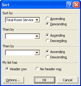
   Figure 3-1: The Sort dialog box.

8. Compare your results to Figure 3-2. Edgar has the highest total room service charges, $1,835.40 in August.

   
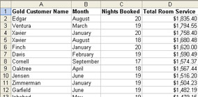
   Figure 3-2: Customers sorted by highest room service charges in descending order.

Note

Although you can sort cells by selecting the cells you want to sort and clicking the Sort Ascending button or Sort Descending button on the Standard toolbar, you might not get the sorting results that you expect.

Filtering Data

Filtering data is an ideal data analysis technique when you want to display a group of records that match specific conditions and hide records that don’t match. (Data is not deleted from hidden rows.) For instance, you may want to find out how many customers purchased a particular product or service or how many products or services came from a particular supplier.

Filtering data is similar to sorting, but filtering displays only the data that matches the filter conditions. You should use filtering when you want to focus your attention on specific records that match your filter conditions.

Filter conditions (also known as filter criteria) can be simple (values in your worksheet) or advanced (criteria that you enter separate from the data values in your worksheet). To filter records in the active worksheet by using simple filter criteria, click any cell in the list of records. Then, on the Data menu, point to Filter, click AutoFilter, and select one of the choices in the AutoFilter lists. The arrow in a cell turns blue to confirm that data is being filtered by criteria selected in that column. You can apply another filter to the data that remains if you want to select even more specific records. If none of the list’s choices meet your needs, you can select Custom from the AutoFilter list to display the Custom AutoFilter dialog box, in which you can specify your own filter criteria. You can use the ? and * characters to represent single and multiple “wildcard” characters, respectively, in custom filter criteria expressions. You can also click the And or Or options to specify whether matching records must meet two criteria or either of the custom filter criteria you enter.

Your Turn

In this exercise, you want to find records for all of the room service charges in August for your preferred customers. Because this group of records is related by containing an identical data value in a specific field, this task is a good candidate for a filtering operation.

1. Open Hotel.xls. If the file is open already, close it without saving the file and open it again.

2. On the Data menu, point to Filter and then click AutoFilter.

3. In cell B1, the Month column, click the arrow and then click August. Only the records for August are displayed. Your results should look similar to Figure 3-3.

   
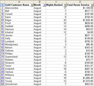
   Figure 3-3: The August data records.

Note

The row numbers in your spreadsheet might not match the row numbers in Figure 3-3. The data should be the same, however.

Tip

To remove filters from the active worksheet, on the Data menu, point to Filter and then click Show All. To remove all filters from the active worksheet and remove the arrows next to each of the row’s cells, point to Filter on the Data menu and then click AutoFilter.

As you experiment with filtering, you might discover some cases in which you aren’t able to use either the AutoFilter list or the Custom AutoFilter dialog box to set up the exact combination of filter criteria that you need. In these cases, you should specify advanced filter criteria. To filter a list of records by using advanced filter criteria, you first need to insert at least three blank rows above the list to which you want to apply the filter.

Tip

A list to which you apply advanced filter criteria must contain a header row. Also, leave at least one blank row between the group of cells making up the advanced filter criteria and the header row of the list to which you want to apply the filter. Otherwise, Excel might not be able to determine where your filter criteria ends and the list of records begins.

After you have inserted the blank rows, in separate cells in the first blank row, type the name of each column by which you want to filter. Then, in the second and subsequent rows, type the advanced filter criteria. Click any cell in the list to which you want to apply the filter criteria, point to Filter on the Data menu, and then click Advanced Filter. Finally, provide the filter criteria in the Advanced Filter dialog box and click OK to apply the filter.

Your Turn

In this exercise, you want to move some of your Gold customers to Platinum status by finding out which customers booked more than 15 nights and spent more than $1,500.00 on room service in any single month during the first quarter of the year. Because these filter criteria involve ranges of potential data values, this is a typical task for an advanced filter.

1. Open the Hotel.xls file. If the file is open already, close it (do not save the file) and then open the file again.

2. Insert five blank rows above the data list. To do so, select cells A1 through A5 and then click Rows on the Insert menu.

3. Type the information shown in Figure 3-4 into cells A1 through C4.

   
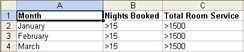
   Figure 3-4: Advanced filter criteria.

4. Click cell A6, and then, on the Data menu, point to Filter and click Advanced Filter.

5. In the List Range box, leave the default value of $A$6:$D$318.

6. Click in the Criteria Range box, and then select cells A1 through C4, inclusive. Compare your results to Figure 3-5.

   
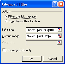
   Figure 3-5: The Advanced Filter dialog box.

7. Click OK. The customers that booked more than 15 nights and spent more than $1,500.00 in any single month during the first quarter of the year include Davis, Finch, Ventura, Xavier, and Zimmerman, as shown in Figure 3-6.

   
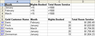
   Figure 3-6: Results of running the advanced filter.

Here are additional advanced filters that you can try:

• Customers that booked less than 5 nights or more than 15 nights in any given month. (See Figure 3-7.)

  
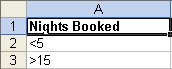
  Figure 3-7: Advanced criteria for customers that booked less than 5 or more than 15 nights in any given month.

• Customers that booked less than 5 nights or more than 15 nights and spent less than $100.00 or more than $1,500.00 on room service in any given month. (See Figure 3-8.)

  
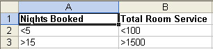
  Figure 3-8: Advanced criteria for customers that booked less than 5 or more than 15 nights and spent less than $100.00 or more than $1,500.00 on room service in any given month.

Putting It Together

You can use a combination of filtering and sorting to quickly reduce the amount of visual clutter while at the same time organizing the data you want to analyze. In the last three exercises, you practiced sorting and filtering data as separate data analysis tasks. In this exercise, you’ll combine sorting and filtering to find out which customer had the highest total room service charge in February. You want to display only the February room service totals and rank the totals in descending order.

1. Open the Hotel.xls file. If the file is open already, close it (do not save the file) and open the file again.

2. On the Data menu, point to Filter and then click AutoFilter.

3. Click the arrow in cell B1, the Month column, and then click February.

4. Select all of the records by pressing CTRL+A.

5. On the Data menu, click Sort.

6. Click the Header Row option.

7. In the Sort By list, select Total Room Service and then click OK.

   Customer Davis had the highest February total room service charge ($1,590.49).