7.3 Reasoning about Probability: The Measurable Case
|
7.3 Reasoning about Probability: The Measurable Case
Reasoning about probability can be formalized along lines similar to those used for reasoning about knowledge. An interpretation π can be added to a probability frame to obtain a probability structure. This gives the appropriate semantic model. Let ![]() probn be the class of probability structures. An important special case is a structure where, at each point, all sets are measurable (i.e.,
probn be the class of probability structures. An important special case is a structure where, at each point, all sets are measurable (i.e., ![]() w,i = 2W w,i for all worlds w and agents i). Let
w,i = 2W w,i for all worlds w and agents i). Let ![]() measn be the class of all measurable probability structures. It is convenient occasionally to be able to talk about simple probability structures. These are the obvious analogues of simple probability frames and have the form (W,
measn be the class of all measurable probability structures. It is convenient occasionally to be able to talk about simple probability structures. These are the obvious analogues of simple probability frames and have the form (W, ![]() , μ, π): that is, a probability space with an associated interpretation.
, μ, π): that is, a probability space with an associated interpretation.
This takes care of the semantics. What about the syntax? I consider a language with likelihood terms of the form ℓi(Φ). The ℓ stands for likelihood. For this section, ℓ(Φ) should be interpreted as "the probability of φ according to agent i." In later sections, the φ is interpreted as "belief" or "plausibility" or "possibility," depending on the notion of likelihood being considered. For this section, I allow linear combinations of likelihood terms, such as 2ℓ(Φ) + 3ℓ(ψ). This makes sense for probability (and possibility), where ℓ(Φ) and ℓ(ψ) are real numbers that can be added, but not for plausibility measures. I later consider a language that allows only comparison of likelihoods and makes sense for all the representation methods. Using the addition operator, it is possible to say, for example, that the probability of the union of two disjoint sets is the sum of their individual probabilities. Linear combinations make it possible to express expectation, for example.
The formal syntax is quite straightforward. Formulas are formed by starting with a set ∊ of primitive propositions and closing off under conjunction, negation, and the formation of (linear) likelihood formulas; a likelihood formula has the form a1ℓ1(Φ1) + … + akℓik (Φk)>b, where a1, …, ak, b are real numbers, i1, …, ik are (not necessarily distinct) agents, and φ1, …, φk are formulas. Thus, a linear likelihood formula talks about a linear combination of likelihood terms of the form ℓi(Φ). For example, 2ℓ1(p1 ∧ p2) + 7ℓ1(p1 ∨ p3) ≥ 3 is a likelihood formula. Since nesting is allowed, so is ℓ1(ℓ2(p) = 1/2) = 1/2. ![]() QUn (Φ) (the QU stands for quantitative uncertainty) is the language that results from starting with Φ and closing off under conjunction, negation, and the formation of likelihood formulas for n agents (i.e., using ℓ1, …, ℓn).
QUn (Φ) (the QU stands for quantitative uncertainty) is the language that results from starting with Φ and closing off under conjunction, negation, and the formation of likelihood formulas for n agents (i.e., using ℓ1, …, ℓn).
![]() QUn (as usual, I suppress Φ) is rich enough to express many notions of interest. For example, I use obvious abbreviations such as
QUn (as usual, I suppress Φ) is rich enough to express many notions of interest. For example, I use obvious abbreviations such as
-
ℓi(Φ) − ℓi(ψ)>b for ℓi(Φ) + (−1)ℓi(ψ)>b,
-
ℓi(Φ)>ℓi(ψ) for ℓi(Φ) − ℓi(ψ) > 0,
-
ℓi(Φ)<ℓi(ψ) for ℓi(ψ) − ℓi(Φ) > 0,
-
ℓi(Φ) ≤ b for (ℓi(Φ)>b),
-
ℓi(Φ) ≥ b for −ℓi(Φ) ≤−b,
-
ℓi(Φ) = b for (ℓi(Φ) ≥ b) ∧ (ℓi(Φ) ≤ b).
Simple conditional probabilities such as ℓi(Φ | ψ) ≥ 2/3 can also be expressed in ![]() QUn. Since ℓi(Φ | ψ) = ℓi(Φ ∧ ψ)/ℓi(ψ), after clearing the denominator, this becomes 3ℓi(Φ ∧ ψ) ≥ 2ℓi(ψ).
QUn. Since ℓi(Φ | ψ) = ℓi(Φ ∧ ψ)/ℓi(ψ), after clearing the denominator, this becomes 3ℓi(Φ ∧ ψ) ≥ 2ℓi(ψ).
As I mentioned earlier, the expected value of a random variable can also be expressed in ![]() QUn, provided that the worlds in which the random variable takes on a particular value can be characterized by formulas. For example, suppose that you win $2 if a coin lands heads and lose $3 if it lands tails. Then your expected winnings are 2ℓ(heads) − 3ℓ(tails). The formula 2ℓ(heads) − 3ℓ(tails) ≥ 1 says that your expected winnings are at least $1.
QUn, provided that the worlds in which the random variable takes on a particular value can be characterized by formulas. For example, suppose that you win $2 if a coin lands heads and lose $3 if it lands tails. Then your expected winnings are 2ℓ(heads) − 3ℓ(tails). The formula 2ℓ(heads) − 3ℓ(tails) ≥ 1 says that your expected winnings are at least $1.
Although ![]() QUn is a very expressive language, it cannot express some important notions. One example is independence. Informally, (after expanding and clearing the denominators) the fact that φ is independent of ψ according to agent i corresponds to the formula ℓi(Φ ∧ ψ) = ℓi(Φ) ℓi(ψ). There is no difficulty giving to semantics such formulas in the semantic framework I am about to describe. However, this formula is not in the language, since I have not allowed multiplication of likelihood terms in linear likelihood formulas. I return to this issue in Section 7.7.
QUn is a very expressive language, it cannot express some important notions. One example is independence. Informally, (after expanding and clearing the denominators) the fact that φ is independent of ψ according to agent i corresponds to the formula ℓi(Φ ∧ ψ) = ℓi(Φ) ℓi(ψ). There is no difficulty giving to semantics such formulas in the semantic framework I am about to describe. However, this formula is not in the language, since I have not allowed multiplication of likelihood terms in linear likelihood formulas. I return to this issue in Section 7.7.
So why not include such formulas in the language? There is a tradeoff here: added expressive power comes at a price. Richer languages are typically harder to axiomatize, and it is typically harder to determine the validity of formulas in a richer language. (See the notes to this chapter for further discussion of this issue and references.) Thus, I stick to the simpler language in this book, for purposes of illustration.
Formulas in ![]() QUn are either true or false at a world in a probability structure; they do not get "probabilistic" truth values. A logic for reasoning about probability can still be two-valued! In this section, I focus on measurable probability structures; this makes life simpler. In a measurable probability structure M, the term ℓi(Φ) is interpreted as the probability (according to agent i) of the set [[φ]]M. But if this set is not measurable, it does not make sense to talk about its probability. As long as all sets are measurable, this problem does not arise. (I consider the case where sets are not necessarily measurable in Section 7.4.)
QUn are either true or false at a world in a probability structure; they do not get "probabilistic" truth values. A logic for reasoning about probability can still be two-valued! In this section, I focus on measurable probability structures; this makes life simpler. In a measurable probability structure M, the term ℓi(Φ) is interpreted as the probability (according to agent i) of the set [[φ]]M. But if this set is not measurable, it does not make sense to talk about its probability. As long as all sets are measurable, this problem does not arise. (I consider the case where sets are not necessarily measurable in Section 7.4.)
Defining the truth of formulas in a measurable probability structure M = (W, 풫![]() 1, …, 풫
1, …, 풫![]() n, π) is straightforward. The definition in the case of primitive propositions, conjunctions, and negations is identical to that for propositional logic. For likelihood formulas,
n, π) is straightforward. The definition in the case of primitive propositions, conjunctions, and negations is identical to that for propositional logic. For likelihood formulas,
![]()
where 풫![]() ij(w) = (Ww,ij,μw,ij).
ij(w) = (Ww,ij,μw,ij).
Example 7.3.1
Suppose that M1 = (W, 2W, μ, π) is a simple probability structure, where
-
W = {w1, w2, w3, w4};
-
μ(w1) = μ(w2) = .25, μ(w3) = .3, μ(w4) = .2; and
-
π is such that (M1, w1) ⊨ p ∧ q, (M1, w2) ⊨ p ∧ q, (M1, w3) ⊨ p ∧ q, and (M1, w4) ⊨ p ∧ q.
Thus, the worlds in W correspond to the four possible truth assignments to p and q.
The structure M1 is described in Figure 7.2.
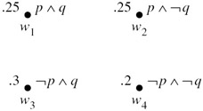
Figure 7.2: The simple probability structure M1.
It is straightforward to check that, for example,
![]()
Even though p ∧ q is true at w1, the agent considers p ∧ q to be more probable than p ∧ q. In addition,
![]()
equivalently, sticking closer to the syntax of ![]() QUn
QUn
![]()
Example 7.3.2
Let M2 = (W, 풫![]() 1, 풫
1, 풫![]() 2), where W, π, and 풫
2), where W, π, and 풫![]() 1 are as in the structure M1 in Example 7.3.1, and 풫
1 are as in the structure M1 in Example 7.3.1, and 풫![]() 2(w1) 풫
2(w1) 풫![]() 2(w2) = ({w1, w2}, μ′1, where μ′1(w1) = .6 and μ′1(w2) = .4, and 풫
2(w2) = ({w1, w2}, μ′1, where μ′1(w1) = .6 and μ′1(w2) = .4, and 풫![]() 2(w3) 풫
2(w3) 풫![]() 2(w4) = ({w3, w4}, μ′2), where μ′2(w3) = μ′2(w4) = .5. The structure M2 is described in Figure 7.3.
2(w4) = ({w3, w4}, μ′2), where μ′2(w3) = μ′2(w4) = .5. The structure M2 is described in Figure 7.3.
It is straightforward to check that, for example,
![]()
At world w1, agent 1 thinks that p and p are equally likely, while agent 2 is certain that p is true. Moreover, agent 2 is certain that agent 1 thinks that p and p are equally likely, while agent 1 is certain that agent 2 ascribes p either probability 0 or probability 1.
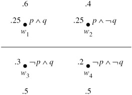
Figure 7.3: The probability structure M2.
I next present a complete axiomatization for reasoning about probability. The system, called AXprobn, divides nicely into three parts, which deal respectively with propositional reasoning, reasoning about linear inequalities, and reasoning about probability. It consists of the following axioms and inference rules, which hold for i = 1, …, n:
-
Propositional reasoning:
-
Prop. All substitution instances of tautologies of propositional logic.
-
MP. From φ and φ ⇒ ψ infer ψ (Modus Ponens).
-
Reasoning about probability:
-
QU1. ℓi(Φ) ≥ 0.
-
QU2. ℓi(true) = 1.
-
QU3. ℓi(Φ ∧ ψ) + ℓi(Φ ∧ ψ) = ℓi(Φ).
-
QUGen. From ℓ ⇔ ψ infer ℓi(ℓ) = ℓi(ψ).
-
Reasoning about linear inequalities:
-
Ineq. All substitution instances of valid linear inequality formulas. (Linear in-equality formulas are discussed shortly.)
Prop and MP should be familiar from the systems Kn in Section 7.2.3. However, note that Prop represents a different collection of axioms in each system, since the underlying language is different in each case. For example, (ℓ1(p) > 0 ∧ (ℓ1(p) > 0)) is an instance of Prop in AXprobn, obtained by substituting formulas in the language ![]() QUn into the propositional tautology (p ∧ p). It is not an instance of Prop in Kn, since this formula is not even in the language
QUn into the propositional tautology (p ∧ p). It is not an instance of Prop in Kn, since this formula is not even in the language ![]() Kn. Axioms QU1–3 correspond to the properties of probability: every set gets nonnegative probability (QU1), the probability of the whole space is 1 (QU2), and finite additivity (QU3). The rule of inference QUGen is an analogue to the generalization rule Gen from Section 7.2. The most obvious analogue is perhaps
Kn. Axioms QU1–3 correspond to the properties of probability: every set gets nonnegative probability (QU1), the probability of the whole space is 1 (QU2), and finite additivity (QU3). The rule of inference QUGen is an analogue to the generalization rule Gen from Section 7.2. The most obvious analogue is perhaps
-
QUGen′. From φ infer ℓi(Φ) = 1.
QUGen′ is provable from QUGen and QU2, but is actually weaker than QUGen and does not seem strong enough to give completeness. For example, it is almost immediate that ℓ1(p) = 1/3 ⇒ℓ1(p ∧ p) = 1/3 is provable using QUGen, but it does not seem to be provable using QUGen′.
The axiom Ineq consists of "all substitution instances of valid linear inequality formulas." To make this precise, let X be a fixed infinite set of variables. A (linear) in-equality term (over X) is an expression of the form a1x1 + … + akxk, where a1, …, ak are real numbers, x1, …, xk are variables in X, and k ≥ 1. A basic (linear) inequality formula is a statement of the form t ≥ b, where t is an inequality term and b is a real number. For example, 2x3 + 7x2 ≥ 3 is a basic inequality formula. A (linear) inequality formula is a Boolean combination of basic inequality formulas. I use f and g to refer to inequality formulas. An assignment to variables is a function A that assigns a real number to every variable. It is straightforward to define the truth of inequality formulas with respect to an assignment A to variables. For a basic inequality formula,
![]()
The extension to arbitrary inequality formulas, which are just Boolean combinations of basic inequality formulas, is immediate:
![]()
As usual, an inequality formula f is valid if A ⊨ f for all assignments A to variables.
A typical valid inequality formula is
![]()
To get an instance of Ineq, simply replace each variable xj that occurs in a valid formula about linear inequalities with a likelihood term ℓij(Φj). (Of course, each occurrence of the variable xj must be replaced by the same primitive likelihood term ℓij (Φj).) Thus, the following likelihood formula, which results from replacing each occurrence of xj in (7.1) by ℓij (Φj), is an instance of Ineq:
![]()
There is an elegant sound and complete axiomatization for Boolean combinations of linear inequalities; however, describing it is beyond the scope of this book (see the notes for a reference). The axiom Ineq gives a proof access to all the valid formulas of this logic, just as Prop gives a proof access to all valid propositional formulas.
The following result says that AXprobn completely captures probabilistic reasoning, to the extent that it is expressible in the language ![]() QUn.
QUn.
Theorem 7.3.3
AXprobn is a sound and complete axiomatization with respect to ![]() measn for the language
measn for the language ![]() QUn
QUn
Proof Soundness is straightforward (Exercise 7.8). The completeness proof is beyond the scope of this book.
What happens in the case of countably additive probability measures? Actually, nothing changes. Let ![]() meas,cn be the class of all measurable probability structures where the probability measures are countably additive. AXprobn is also a sound and complete axiomatization with respect to
meas,cn be the class of all measurable probability structures where the probability measures are countably additive. AXprobn is also a sound and complete axiomatization with respect to ![]() meas,cn for the language
meas,cn for the language ![]() QUn. Intuitively, this is because the language
QUn. Intuitively, this is because the language ![]() QUn cannot distinguish between finite and infinite structures. It can be shown that if a formula in
QUn cannot distinguish between finite and infinite structures. It can be shown that if a formula in ![]() QUn is satisfiable at all, then it is satisfiable in a finite structure. Of course, in finite structure, countable additivity and finite additivity coincide. Thus, no additional axioms are needed to capture countable additivity. For similar reasons, there is no need to attempt to axiomatize continuity properties for the other representations of uncertainty considered in this chapter.
QUn is satisfiable at all, then it is satisfiable in a finite structure. Of course, in finite structure, countable additivity and finite additivity coincide. Thus, no additional axioms are needed to capture countable additivity. For similar reasons, there is no need to attempt to axiomatize continuity properties for the other representations of uncertainty considered in this chapter.
|
EAN: 2147483647
Pages: 140