6.3 Multi-Agent Systems

6.3 Multi-Agent Systems

Frames as presented in the previous two sections are static. In this section, I introduce multi-agent systems, which incorporate time and give worlds more structure. I interpret the phrase "multi-agent system" rather loosely. Players in a poker game, agents conducting a bargaining session, robots interacting to clean a house, and processes performing a distributed computation can all be viewed as multi-agent systems. The only assumption I make here about a system is that, at all times, each of the agents in the system can be viewed as being in some local or internal state. Intuitively, the local state encapsulates all the relevant information to which the agent has access. For example, in a poker game, a player's state might consist of the cards he currently holds, the bets made by the other players, any other cards he has seen, and any information he may have about the strategies of the other players (e.g., Bob may know that Alice likes to bluff, while Charlie tends to bet conservatively). These states could have further structure (and typically will in most applications of interest). In particular, they can often be characterized by a set of random variables.

It is also useful to view the system as a whole as being in a state. The first thought might be to make the system's state be a tuple of the form (s₁,…, s_n), where s_i is agent i's state. But, in general, more than just the local states of the agents may be relevant to an analysis of the system. In a message-passing system where agents send messages back and forth along communication lines, the messages in transit and the status of each communication line (whether it is up or down) may also be relevant. In a system of sensors observing some terrain, features of the terrain may certainly be relevant. Thus, the system is conceptually divided into two components: the agents and the environment, where the environment can be thought of as "everything else that is relevant." In many ways the environment can be viewed as just another agent. A global state of a system with n agents is an (n + 1)-tuple of the form (s_e, s₁,…, s_n), where s_e is the state of the environment and s_i is the local state of agent i.

A global state describes the system at a given point in time. But a system is not a static entity. It is constantly changing over time. A run captures the dynamic aspects of a system. Intuitively, a run is a complete description of one possible way in which the system's state can evolve over time. Formally, a run is a function from time to global states. For definiteness, I take time to range over the natural numbers. Thus, r(0) describes the initial global state of the system in a possible execution, r(1) describes the next global state, and so on. A pair (r, m) consisting of a run r and time m is called a point. If r(m) = (s_e, s₁,…, s_n), then define r_e(m) = s_e and r_i(m) = s_i, i = 1,…, n; thus, r_i(m) is agent i's local state at the point (r, m) and r_e(m) is the environment's state at (r, m).

Typically global states change as a result of actions. Round m takes place between time m − 1 and m. I think of actions in a run r as being performed during a round. The point (r, m − 1) describes the situation just before the action at round m is performed, and the point (r, m) describes the situation just after the action has been performed.

In general, there are many possible executions of a system: there could be a number of possible initial states and many things that could happen from each initial state. For example, in a draw poker game, the initial global states could describe the possible deals of the hand by having player i's local state describe the cards held by player i. For each fixed deal of the cards, there may still be many possible betting sequences, and thus many runs. Formally, a system is a nonempty set of runs. Intuitively, these runs describe all the possible sequences of events that could occur in the system. Thus, I am essentially identifying a system with its possible behaviors.

Although a run is an infinite object, there is no problem representing a finite process (e.g., a finite protocol or finite game) using a system. For example, there could be a special global state denoting that the protocol/game has ended, or the final state could be repeated infinitely often. These are typically minor modeling issues.

A system (set of runs) can be identified with an epistemic frame = (W, ₁, …, _n), where the _is are equivalence relations. The worlds in are the points in , that is, the pairs (r, m) such that r ∈ . If s = (s_e, s₁,…, s_n) and s′ = (s′_e, s′₁,…, s′_n) are two global states in , then s and s′ are indistinguishable to agent i, written s ~_i s′, if i has the same state in both s and s′, that is, if s_i = s′_i. The indistinguishability relation ~_i can be extended to points. Two points (r, m) and (r′, m′) are indistinguishable to i, written (r, m) ~_i (r′, m′), if r(m) ~_i r′(m′) (or, equivalently, if r_i(m) = r′_i(m′)). Clearly ~_i is an equivalence relation on points; take the equivalence relation _i of F to be ~_i. Thus, _i(r, m) = {(r′, m′) : r_i(m) = r′_i(m′)}, the set of points indistinguishable by i from (r, m).

To model a situation as a multi-agent system requires deciding how to model the local states. The same issues arise as those discussed in Section 2.1: what is relevant and what can be omitted. This, if anything, is an even harder task in a multi-agent situation than it is in the single-agent situation, because now the uncertainty includes what agents are thinking about one another. This task is somewhat alleviated by being able to separate the problem into considering the local state of each agent and the state of the environment. Still, it is by no means trivial. The following simple example illustrates some of the subtleties that arise:

Example 6.3.1

Suppose that Alice tosses two coins and sees how the coins land. Bob learns how the first coin landed after the second coin is tossed, but does not learn the outcome of the second coin toss. How should this be represented as a multi-agent system? The first step is to decide what the local states look like. There is no "right" way of modeling the local states. What I am about to describe is one reasonable way of doing it, but clearly there are others.

The environment state will be used to model what actually happens. At time 0, it is 〈〉, the empty sequence, indicating that nothing has yet happened. At time 1, it is either 〈H 〉 or 〈T 〉, depending on the outcome of the first coin toss. At time 2, it is either 〈H, H 〉, 〈H, T 〉, 〈T, H 〉,or 〈T, T 〉, depending on the outcome of both coin tosses. Note that the environment state is characterized by two random variables, describing the outcome of each coin toss. Since Alice knows the outcome of the coin tosses, I take Alice's local state to be the same as the environment state at all times.

What about Bob's local state? After the first coin is tossed, Bob still knows nothing; he learns the outcome of the first coin toss after the second coin is tossed. The first thought might then be to take his local states to have the form 〈〉 at time 0 and time 1 (since he does not know the outcome of the first coin toss at time 1) and either 〈H 〉 or 〈T 〉 at time 2. This would be all right if Bob cannot distinguish between time 0 and time 1; that is, if he cannot tell when Alice tosses the first coin. But if Bob is aware of the passage of time, then it may be important to keep track of the time in his local state. (The time can still be ignored if it is deemed irrelevant to the analysis. Recall that I said that the local state encapsulates all the relevant information to which the agent has access. Bob has all sorts of other information that I have chosen not to model: his sister's name, his age, the color of his car, and so on. It is up to the modeler to decide what is relevant here.) In any case, if the time is deemed to be relevant, then at time 1, Bob's state must somehow encode the fact that the time is 1. I do this by taking Bob's state at time 1 to be 〈tick〉, to denote that one time tick has passed. (Other ways of encoding the time are, of course, also possible.) Note that the time is already implicitly encoded in Alice's state: the time is 1 if and only if her state is either 〈H 〉 or 〈T 〉.

Under this representation of global states, there are seven possible global states:

• (〈〉, 〈〉, 〈〉), the initial state,

• two time-1 states of the form (〈X₁〉, 〈X₁〉, 〈tick〉), for X₁ ∈ {H, T },

• four time-2 states of the form (〈X₁, X₂〉, 〈X₁, X₂〉, 〈tick, X₁〉), for X₁, X₂ ∈ {H, T }.

In this simple case, the environment state determines the global state (and is identical to Alice's state), but this is not always so.

The system describing this situation has four runs, r¹,…, r⁴, one for each of the time-2 global states. The runs are perhaps best thought of as being the branches of the computation tree described in Figure 6.3.

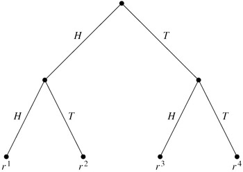
Figure 6.3: Tossing two coins.

Example 6.3.1 carefully avoided discussion of probabilities. There is, of course, no problem adding probability (or any other representation of uncertainty) to the framework. I focus on probability in most of the chapter and briefly discuss the few issues that arise when using nonprobabilistic representations of uncertainty in Section 6.10. A probability system is a tuple (, ₁, …, _n), where is a system and ₁, …, _n are probability assignments; just as in the case of probability frames, the probability assignment _i associates with each point (r, m) a probability space _i(r, m) = (W_r,m,i, _r,m,i, μ_r,m,i).

In the multi-agent systems framework, it is clear where the _i relations that define knowledge are coming from; they are determined by the agents' local states. Where should the probability assignments come from? It is reasonable to expect, for example, that _i(r, m + 1) would somehow incorporate whatever agent i learned at (r, m + 1) but otherwise involve minimal changes from _i(r, m). This suggests the use of conditioning—and, indeed, conditioning will essentially be used—but there are some subtleties involved. It may well be that W_r,m,i and W_{r, m+1,i} are disjoint sets. In that case, clearly μ_{r, m+1,i} cannot be the result of conditioning μ_{r, m,i} on some event. Nevertheless, there is a way of viewing μ_{r, m+1,i} as arising from μ_{r, m,i} by conditioning. The idea is to think in terms of a probability on runs, not points. The following example illustrates the main ideas:

Example 6.3.2

Consider the situation described in Example 6.3.1, but now suppose that the first coin has bias 2/3, the second coin is fair, and the coin tosses are independent, as shown in Figure 6.4. Note that, in Figure 6.4, the edges coming out of each node are labeled with a probability, which is intuitively the probability of taking that transition. Of course, the probabilities labeling the edges coming out of any fixed node must sum to 1, since some transition must be taken. For example, the edges coming out of the root have probability 2/3 and 1/3. Since the transitions in this case (i.e., the coin tosses) are assumed to be independent, it is easy to compute the probability of each run. For example, the probability of run r¹ is 2/3 1/2 = 1/3; this represents the probability of getting two heads.

The probability on runs can then be used to determine probability assignments. Note that in a probability assignment, the probability is put on points, not on runs. Suppose that _i(r^j, m) = (W_r^j,m,i, 2^W_rj,m,i), μ_r^j,m,i. An obvious choice for W_r^j,m,i is _i(r^j,m); the agents ascribe probability to the worlds they consider possible. Moreover, the relative probability of the points is determined by the probability of the runs. For example, W_{r¹, 0, A} = _A(r¹, 0) = {(r¹, 0), (r², 0), (r³, 0), (r⁴, 0)}, and μ_r¹,0,A assigns probability μ_r¹,0,A(r¹,0) = 1/3; similarly, W_{r¹, 2, B} = _B(r¹, 2) = {(r¹, 2), (r², 2)} and μ_{r¹, 2, B}(r¹, 2) = 1/2. Note that to compute μ_{r¹, 2, B}(r¹, 2), Bob essentially takes the initial probability on the runs, and he conditions on the two runs he considers possible at time 2, namely, r¹ and r². It is easy to check that this probability assignment satisfies SDP and CONS. Indeed, as shown in the next section, this is a general property of the construction.

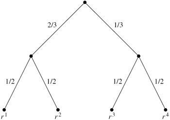
Figure 6.4: Tossing two coins, with probabilities.

As long as there is some way of placing a probability on the set of runs, the ideas in this example generalize. This is formalized in the following section.