5.2 Expectation for Other Notions of Likelihood
|
5.2 Expectation for Other Notions of Likelihood
How should expectation be defined for other representations of uncertainty? I start with sets of probability measures, since the results in this case are fairly straightforward and form the basis for other representations.
5.2.1 Expectation for Sets of Probability Measures
There are straightforward analogues of lower and upper probability in the context of expectation. If ![]() is a set of probability measures such that X is measurable with respect to each probability measure μ ∊
is a set of probability measures such that X is measurable with respect to each probability measure μ ∊ ![]() , then define E
, then define E![]() (X) = {Eμ(X) : μ ∊
(X) = {Eμ(X) : μ ∊ ![]() }. E
}. E![]() (X) is a set of numbers. Define the lower expectation and upper expectation of X with respect to
(X) is a set of numbers. Define the lower expectation and upper expectation of X with respect to ![]() , denoted E
, denoted E![]() (X) and E
(X) and E![]() (X), as the inf and sup of the set E
(X), as the inf and sup of the set E![]() (X), respectively. Clearly
(X), respectively. Clearly ![]() *(U) = E
*(U) = E![]() (XU) and
(XU) and ![]() *(U) = E
*(U) = E![]() (XU). The properties of E
(XU). The properties of E![]() and E
and E![]() are not so different from those of probabilistic expectation.
are not so different from those of probabilistic expectation.
Proposition 5.2.1
The functions E![]() and E
and E![]() have the following properties, for all gambles X and Y.
have the following properties, for all gambles X and Y.
-
E
 is subadditive: E
 (X + Y) ≤ E
 (X) + E
 (Y);
(Y);E
 is superadditive: E
 (X + Y) ≥ E
 (X) + E
 (Y).
(Y). -
E
 and E
and E are both positively affinely homogeneous:

-
E
 and E
and E are monotone.
 -
E
 (X) = − E
 (−X).
(−X).
Proof See Exercise 5.8.
Superadditivity (resp., subadditivity), positive affine homogeneity, and monotonicity in fact characterize E![]() (resp., E
(resp., E![]() ), although the proof of this fact is beyond the scope of the book.
), although the proof of this fact is beyond the scope of the book.
Theorem 5.2.2
Suppose that E maps gambles measurable with respect to ![]() to ℝ and is superadditive (resp., subadditive), positively affinely homogeneous, and monotone. Then there is a set
to ℝ and is superadditive (resp., subadditive), positively affinely homogeneous, and monotone. Then there is a set ![]() of probability measures on
of probability measures on ![]() such that E = E
such that E = E![]() (resp., E = E
(resp., E = E![]() ).
).
(There is another equivalent characterization of E![]() ; see Exercise 5.9.)
; see Exercise 5.9.)
The set ![]() constructed in Theorem 5.2.2 is not unique. It is not hard to construct sets
constructed in Theorem 5.2.2 is not unique. It is not hard to construct sets ![]() and
and ![]() ′ such that
′ such that ![]() ≠
≠ ![]() ′ but E
′ but E![]() = E
= E![]() ′ (see Exercise 5.10). However, there is a canonical largest set
′ (see Exercise 5.10). However, there is a canonical largest set ![]() such that E = E
such that E = E![]() ;
; ![]() consists of all probability measures μ such that Eμ(X) ≥ E(x) for all gambles X.
consists of all probability measures μ such that Eμ(X) ≥ E(x) for all gambles X.
There is also an obvious notion of expectation corresponding to Pl![]() (as defined in Section 2.8). EPl
(as defined in Section 2.8). EPl![]() maps a gamble X to a function fX from
maps a gamble X to a function fX from ![]() to ℝ, where fX(μ) = Eμ(X). This is analogous to Pl
to ℝ, where fX(μ) = Eμ(X). This is analogous to Pl![]() , which maps sets to functions from
, which maps sets to functions from ![]() to [0, 1]. Indeed, it should be clear that EPl
to [0, 1]. Indeed, it should be clear that EPl![]() , so that the relationship between EPl
, so that the relationship between EPl![]() and Pl
and Pl![]() is essentially the same as that between Eμ and μ. Not surprisingly, there are immediate analogues of Proposition 5.1.1 and 5.1.2.
is essentially the same as that between Eμ and μ. Not surprisingly, there are immediate analogues of Proposition 5.1.1 and 5.1.2.
Proposition 5.2.3
The function EPl![]() is additive, affinely homogeneous, and monotone.
is additive, affinely homogeneous, and monotone.
Proof See Exercise 5.13.
Proposition 5.2.4
Suppose that E maps gambles measurable with respect to ![]() to functions from I to ℝ and is additive, affinely homogeneous, and monotone. Then there is a (necessarily unique) set
to functions from I to ℝ and is additive, affinely homogeneous, and monotone. Then there is a (necessarily unique) set ![]() of probability measures on
of probability measures on ![]() indexed by I such that E = EPl
indexed by I such that E = EPl![]() .
.
Proof See Exercise 5.14.
Note that if ![]() ≠
≠ ![]() ′, then EPl
′, then EPl![]() ≠ EPl
≠ EPl![]() ′. As observed earlier, this is not the case with upper and lower expectation; it is possible that
′. As observed earlier, this is not the case with upper and lower expectation; it is possible that ![]() =
= ![]() ′ yet E
′ yet E![]() = E
= E![]() ′ (and hence E
′ (and hence E![]() = E
= E![]() ′). Thus, EPl
′). Thus, EPl![]() can be viewed as capturing more information about
can be viewed as capturing more information about ![]() than E
than E![]() . On the other hand, E
. On the other hand, E![]() captures more information than
captures more information than ![]() *. Since
*. Since ![]() * (U) = E
* (U) = E![]() (U), it is immediate that if
(U), it is immediate that if ![]() * ≠
* ≠ ![]() ′*, then E
′*, then E![]() ≠ E
≠ E![]() ′. However, as Example 5.2.10 shows, there are sets
′. However, as Example 5.2.10 shows, there are sets ![]() and
and ![]() ′ of probability measures such that
′ of probability measures such that ![]() * =
* = ![]() ′* but E
′* but E![]() ≠ E
≠ E![]() *.
*.
As for probability, there are additional continuity properties for E![]() , E
, E![]() , and EPl
, and EPl![]() if
if ![]() consists of countably additive measures. They are the obvious analogues of (5.4) and (5.5).
consists of countably additive measures. They are the obvious analogues of (5.4) and (5.5).
![]()
![]()
![]()
(See Exercise 5.12.) Again, just as with upper and lower probability, the analogue of (5.6) does not hold for lower expectation, and the analogue of (5.7) does not hold for upper expectation. (Indeed, counterexamples for upper and lower probability can be converted to counterexamples for upper and lower expectation by taking indicator functions.) On the other hand, it is easy to see that the analogue of (5.5) does hold for EPl![]() .
.
Analogues of (5.4) and (5.5) hold for all the other notions of expectation I consider if the underlying representation satisfies the appropriate continuity property. To avoid repetition, I do not mention this again.
5.2.2 Expectation for Belief Functions
There is an obvious way to define a notion of expectation based on belief functions, using the identification of Bel with (![]() Bel)* (see Theorem 2.4.1). Given a belief function Bel, define EBel = E
Bel)* (see Theorem 2.4.1). Given a belief function Bel, define EBel = E![]() Bel. Similarly, for the corresponding plausibility function Plaus, define EPlause = E
Bel. Similarly, for the corresponding plausibility function Plaus, define EPlause = E![]() Bel.
Bel.
This is well defined, but, as with the case of conditional belief, it seems more natural to get a notion of expectation for belief functions that is defined purely in terms of belief functions, without reverting to probability. It turns out that this can be done using the analogue of (5.3). If ![]() (X) = {x1,…, xn}, with x1 < … < xn, define
(X) = {x1,…, xn}, with x1 < … < xn, define
![]()
An analogous definition holds for plausibility:
![]()
Proposition 5.2.5
EBel = E′Bel and EPlaus = E′Plaus.
Proof See Exercise 5.15.
Equation (5.9) gives a way of defining expectation for belief and plausibility functions without referring to probability. (Another way of defining expectation for belief functions, using mass functions, is given in Exercise 5.16; another way of defining expected plausibility, using a different variant of (5.2), is given in Exercise 5.17.)
The analogue of (5.2) could, of course, be used to define a notion of expectation for belief functions, but it would not give a very reasonable notion. For example, suppose that W ={a, b} and Bel(a) = Bel(b) = 0. (Of course, Bel({a, b}) = 1.) Consider a gamble X such that X(A) = 1 and X(b) = 2. According to the obvious analogue of (5.1) or (5.2) (which are equivalent in this case), the expected belief of X is 0, since Bel(a) = Bel(b) = 0. However, it is easy to see that EBel(X) = 1 and EPlaus(X) = 2, which seems far more reasonable. The real problem is that (5.2) is most appropriate for plausibility measures that are additive (in the sense defined in Section 2.8; i.e., there is a function ⊕ such that Pl(U ∪ V) = Pl(U) ⊕ Pl(V) for disjoint sets U and V). Indeed, the equivalence of (5.1) and (5.2) depends critically on the fact that probability is additive. As observed in Section 2.8 (see Exercise 2.56), belief functions are not additive. Thus, not surprisingly, using (5.2) does not give reasonable results.
Since EBel can be viewed as a special case of the lower expectation E![]() (taking
(taking ![]() =
= ![]() Bel), it is immediate from Proposition 5.2.1 that EBel is superadditive, positively affinely homogeneous, and monotone. (Similar remarks hold for EPlaus, except that it is subadditive. For ease of exposition, I focus on EBel in the remainder of this section, although analogous remarks hold for EPlaus.) But EBel has additional properties. Since it is immediate from the definition that EBel(XU) = Bel(XU), the inclusion-exclusion property B3 of belief functions can be expressed in terms of expectation (just by replacing all instances of Bel(V) in B3 by EBel(XV)). Moreover, it does not follow from the other properties, since it does not hold for arbitrary lower probabilities (see Exercise 2.14).
Bel), it is immediate from Proposition 5.2.1 that EBel is superadditive, positively affinely homogeneous, and monotone. (Similar remarks hold for EPlaus, except that it is subadditive. For ease of exposition, I focus on EBel in the remainder of this section, although analogous remarks hold for EPlaus.) But EBel has additional properties. Since it is immediate from the definition that EBel(XU) = Bel(XU), the inclusion-exclusion property B3 of belief functions can be expressed in terms of expectation (just by replacing all instances of Bel(V) in B3 by EBel(XV)). Moreover, it does not follow from the other properties, since it does not hold for arbitrary lower probabilities (see Exercise 2.14).
B3 seems like a rather specialized property, since it applies only to indicator functions. There is a more general version of it that also holds for EBel. Given gambles X and Y, define the gambles X ∧ Y and X ∨ Y as the minimum and maximum of X and Y, respectively; that is, (X ∧ Y)(w) = min(X(w), Y(w)) and (X ∨ Y)(w) = max(X(w), Y(w)). Consider the following inclusion-exclusion rule for expectation:
![]()
Since it is immediate that XU∪V = XU ∨ XV and XU∩V = XU ∧ XV, (5.11) generalizes B3.
There is yet another property satisfied by expectation based on belief functions. Two gambles X and Y are said to be comonotonic if it is not the case that one increases while the other decreases; that is, there do not exist worlds w, w′ such that X(w) < X(w′) while Y(w) > Y(w′). Equivalently, there do not exist w and w′ such that (X(w) − X(w′))(Y(w) − Y(w′)) < 0.
Example 5.2.6
Suppose that
-
W ={w1, w2, w3};
-
X(w1) = 1, X(w2) = 3, and X(w3) = 0;
-
Y(w1) = 2, Y(w2) = 7, and Y(w3) = 4;
-
Z(w1) = 3, Z(w2) = 5, and Z(w3) = 3.
Then X and Y are not comonotonic. The reason is that X decreases from w1 to w3, while Y increases from w1 to w3. On the other hand, X and Z are comonotonic, as are Y and Z.
Consider the following property of comonotonic additivity:
![]()
Proposition 5.2.7
The function EBel is superadditive, positively affinely homogeneous, and monotone, and it satisfies (5.11) and (5.12).
Proof The fact that EBel is superadditive, positively affinely homogeneous, and monotone follows immediately from Proposition 5.2.3. The fact that it satisfies (5.11) follows from B3 and Proposition 5.2.5 (Exercise 5.18). Proving that it satisfies (5.12) requires a little more work, although it is not that difficult. I leave the details to the reader (Exercise 5.19).
Theorem 5.2.8
Suppose that E maps gambles to ℝ and E is positively affinely homogeneous, is monotone, and satisfies (5.11) and (5.12). Then there is a (necessarily unique) belief function Bel such that E = EBel.
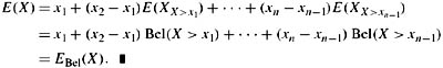
Proof Define Bel(U) = E(XU). Just as in the case of probability, it follows from positive affine homogeneity and monotonicity that Bel(∅) = 0, Bel(W) = 1, and 0 ≤ Bel(U) ≤ 1 for all U ⊆ W. By (5.11) (specialized to indicator functions), it follows that Bel satisfies B3. Thus, Bel is a belief function. Now if X is a gamble such that ![]() (X) = {x1,…,xn} and x1 < x2 < … < xn, define
(X) = {x1,…,xn} and x1 < x2 < … < xn, define
![]()
for j = 1, …, n. It is not hard to show that X = Xn and that Xj and (xj+1 − xj)XX>xj are comonotonic, for j = 1, …, n − 1(Exercise 5.20). Now applying (5.12) repeatedly, it follows that
![]()
Now applying positive affine homogeneity, it follows that
Note that superadditivity was not assumed in the statement of Theorem 5.2.8. Indeed, it is a consequence of Theorem 5.2.8 that superadditivity follows from the other properties. In fact, the full strength of positive affine homogeneity is not needed either in Theorem 5.2.8. It suffices to assume that ![]() .
.
Lemma 5.2.9
Suppose that E is such that (a) ![]() , (b) E is monotone, and (c) E satisfies (5.12). Then E satisfies positive affine homogeneity.
, (b) E is monotone, and (c) E satisfies (5.12). Then E satisfies positive affine homogeneity.
Proof See Exercise 5.21.
It follows easily from these results that EBel is the unique function E mapping gambles to ℝ that is superadditive, positively affinely homogeneous, monotone, and it satisfies (5.11) and (5.12) such that E(XU) = Bel(U) for all U ⊆ W. Proposition 5.2.7 shows that EBel has these properties. If E′ is a function from gambles to ℝ that has these properties, by Theorem 5.2.8, E′ = EBel′ for some belief function Bel′. Since E′(XU) = Bel′(U) = Bel(U) for all U ⊆ W, it follows that Bel = Bel′.
This observation says that Bel and EBel contain the same information. Thus, so do (![]() Bel)* and E
Bel)* and E![]() Bel (since Bel = (
Bel (since Bel = (![]() Bel)* and EBel = E
Bel)* and EBel = E![]() Bel). However, this is not true for arbitrary sets
Bel). However, this is not true for arbitrary sets ![]() of probability measures, as the following example shows:
of probability measures, as the following example shows:
Example 5.2.10
Let W ={1, 2, 3}. A probability measure μ on W can be characterized by a triple (a1, a2, a3), where μ(i) = ai. Let ![]() consist of the three probability measures (0, 3/8, 5/8), (5/8, 0, 3/8), and (3/8, 5/8, 0). It is almost immediate that
consist of the three probability measures (0, 3/8, 5/8), (5/8, 0, 3/8), and (3/8, 5/8, 0). It is almost immediate that ![]() * is 0 on singleton subsets of W and
* is 0 on singleton subsets of W and ![]() * = 3/8 for doubleton subsets. Let
* = 3/8 for doubleton subsets. Let ![]() ′ =
′ = ![]() ′
′ ![]() ∪ {μ4}, where μ4 = (5/8, 3/8, 0). It is easy to check that
∪ {μ4}, where μ4 = (5/8, 3/8, 0). It is easy to check that ![]() ′* =
′* = ![]() *. However, E
*. However, E![]() ≠ E
≠ E![]() ′. In particular, let X be the gamble such that X(1) = 1, X(2) = 2, and X(3) = 3. Then E
′. In particular, let X be the gamble such that X(1) = 1, X(2) = 2, and X(3) = 3. Then E![]() (X) = 13/8, but E
(X) = 13/8, but E![]() ′(X) = 11/8. Thus, although E
′(X) = 11/8. Thus, although E![]() and E
and E![]() ′ agree on indicator functions, they do not agree on all gambles. In light of the earlier discussion, it should be no surprise that
′ agree on indicator functions, they do not agree on all gambles. In light of the earlier discussion, it should be no surprise that ![]() * is not a belief function (Exercise 5.23).
* is not a belief function (Exercise 5.23).
5.2.3 Inner and Outer Expectation
Up to now, I have assumed that all gambles X were measurable, that is, for each x ∊ ![]() (X), the set {w : X(w) = x} was in the domain of whatever representation of uncertainty was being used. But what if X is not measurable? In this case, it seems reasonable to consider an analogue of inner and outer measures for expectation.
(X), the set {w : X(w) = x} was in the domain of whatever representation of uncertainty was being used. But what if X is not measurable? In this case, it seems reasonable to consider an analogue of inner and outer measures for expectation.
The naive analogue is just to replace μ in (5.2) with the inner measure μ* and the outer measure μ*, respectively. Let E?μ and E?μ denote these notions of inner and outer expectation, respectively. As the notation suggests, defining inner and outer expectation in this way can lead to intuitively unreasonable answers. In particular, these functions are not monotone, as the following example shows:
Example 5.2.11
Consider a space W = {w1, w2} and the trivial algebra ![]() = { W}. Let μ be the unique (trivial) probability measure on
= { W}. Let μ be the unique (trivial) probability measure on ![]() . Suppose that X1, X2, and X3 are gambles such that X1(w1) = X1(w2) = 1, X3(w1) = X3(w2) = 2, and X2(w1) = 1 and X2(w2) = 2. Clearly, X1 ≤ X2 ≤ X3. Moreover, it is immediate from the definitions that E?μ(X1) = 1 and E?μ(X3) = 2. However, E?μ(X2) = 0, since μ*(w1) = μ*(w2) = 0, and E?μ(X2) = 3, since μ*(w1) = μ*(w2) = 1. Thus, neither Eμ? nor Eμ? is monotone.
. Suppose that X1, X2, and X3 are gambles such that X1(w1) = X1(w2) = 1, X3(w1) = X3(w2) = 2, and X2(w1) = 1 and X2(w2) = 2. Clearly, X1 ≤ X2 ≤ X3. Moreover, it is immediate from the definitions that E?μ(X1) = 1 and E?μ(X3) = 2. However, E?μ(X2) = 0, since μ*(w1) = μ*(w2) = 0, and E?μ(X2) = 3, since μ*(w1) = μ*(w2) = 1. Thus, neither Eμ? nor Eμ? is monotone.
Note that it is important that E?μ and Eμ? are defined using (5.2), rather than (5.1). If (5.1) were used then, for example, E?μ and Eμ? would be monotone. On the other hand, E?μ(X1) would be 0. Indeed, E?μ(Y) would be 0 for every gamble Y. This certainly is not particularly reasonable either!
Since an inner measure is a belief function, the discussion of expectation for belief suggests two other ways of defining inner and outer expectation.
-
The first uses sets of probabilities. As in Section 2.3, given a probability measure μ defined on an algebra
 ′ that is a subalgebra of
  , let
, let  μ consist of all the extensions of μ to
  . Recall from Theorem 2.3.3 that μ*(U) = (
 μ)*(U) and μ*(U) = (
 μ)* for all U ∊
  . Define Eμ = E
 μ and Eμ = E
 μ.
μ. -
The second approach uses (5.3); define E′μ and Eμ′ by replacing the μ in (5.3) by μ* and μ*, respectively.
In light of Proposition 5.2.5, the following should come as no surprise:
Proposition 5.2.12
Eμ = E′μ and Eμ = Eμ′.
Proof Since it is immediate from the definitions that ![]() μ is
μ is ![]() Bel for Bel = μ*, the fact that Eμ = Eμ′ is immediate from Proposition 5.2.5. It is immediate from Proposition 5.2.1(d) and the definition that Eμ(X) =−Eμ(−X). It is easy to check that Eμ′(X) =−E′μ(−X) (Exercise 5.24). Thus, Eμ = Eμ′.
Bel for Bel = μ*, the fact that Eμ = Eμ′ is immediate from Proposition 5.2.5. It is immediate from Proposition 5.2.1(d) and the definition that Eμ(X) =−Eμ(−X). It is easy to check that Eμ′(X) =−E′μ(−X) (Exercise 5.24). Thus, Eμ = Eμ′.
Eμ has much more reasonable properties than E?μ. (Since Eμ(X) =−Eμ(−X), the rest of the discussion is given in terms of Eμ.) Indeed, since μ* is a belief function, Eμ is superadditive, positively affinely homogeneous, and monotone, and it satisfies (5.11) and (5.12). But Eμ has an additional property, since it is determined by a probability measure. If μ is a measure on ![]() , then the lower expectation of a gamble Y can be approximated by the lower expectation of random variables measurable with respect to
, then the lower expectation of a gamble Y can be approximated by the lower expectation of random variables measurable with respect to ![]() .
.
Lemma 5.2.13
If μ is a probability measure on an algebra ![]() , and X is a gamble measurable with respect to an algebra
, and X is a gamble measurable with respect to an algebra ![]() ′ ⊇
′ ⊇ ![]() , then Eμ(X) = sup{Eμ(Y) : Y ≤ X, Y is measurable with respect to
, then Eμ(X) = sup{Eμ(Y) : Y ≤ X, Y is measurable with respect to ![]() }.
}.
Proof See Exercise 5.25.
To get a characterization of Eμ, it is necessary to abstract the property characterized in Lemma 5.2.13. Unfortunately, the abstraction is somewhat ugly. Say that a function E on ![]() ′-measurable gambles is determined by
′-measurable gambles is determined by ![]() ⊆
⊆ ![]() ′ if
′ if
-
for all
 ′-measurable gambles X, E(x) = sup{E(Y) : Y ≤ X, Y is measurable with respect to
  },
}, -
E is additive for gambles measurable with respect to
 (so that E(x + Y) = E(x) + E(Y) if X and Y are measurable with respect to
  .
.
Theorem 5.2.14
Suppose that E maps gambles measurable with respect to ![]() to ℝ and is positively affinely homogeneous, is monotone, and satisfies (5.11) and (5.12), and there is some
to ℝ and is positively affinely homogeneous, is monotone, and satisfies (5.11) and (5.12), and there is some ![]() ⊆
⊆ ![]() ′ such that E is determined by
′ such that E is determined by ![]() . Then there is a unique probability measure μ on
. Then there is a unique probability measure μ on ![]() such that E = Eμ.
such that E = Eμ.
Proof See Exercise 5.26.
5.2.4 Expectation for Possibility Measures and Ranking Functions
Since a possibility measure can be viewed as a plausibility function, expectation for possibility measures can be defined using (5.10). It follows immediately from Poss3 that the expectation EPoss defined from a possibility measure Poss in this way satisfies the sup property:
![]()
Proposition 5.2.15
The function EPoss is positively affinely homogeneous, is monotone, and satisfies (5.12) and (5.13).
Proof See Exercise 5.27.
I do not know if there is a generalization of (5.13) that can be expressed using arbitrary gambles, not just indicator functions. The obvious generalization—EPoss(X ∨ Y) = max(EPoss(X), EPoss(Y))—is false (Exercise 5.28). In any case, (5.13) is the extra property needed to characterize expectation for possibility.
Theorem 5.2.16
Suppose that E is a function on gambles that is positively affinely homogeneous, is monotone, and satisfies (5.12) and (5.13). Then there is a (necessarily unique) possibility measure Poss such that E = EPoss.
Proof See Exercise 5.29.
Note that, although Poss is a plausibility function, and thus satisfies the analogue of (5.11) with ≥ replaced by ≤ and ∨ switched with ∧, there is no need to state this analogue explicitly; it follows from (5.13). Similarly, subadditivity follows from the other properties. (Since a possibility measure is a plausibility function, not a belief function, the corresponding expectation is subadditive rather than superadditive.)
While this definition of EPoss makes perfect sense and, as Theorem 5.2.16 shows, has an elegant characterization, it is worth noting that there is somewhat of a mismatch between the use of max in relating Poss(U ∪ V), Poss(U), and Poss(V) (i.e., using max for ⊕) and the use of + in defining expectation. Using max instead of + gives a perfectly reasonable definition of expectation for possibility measures (see Exercise 5.30). However, going one step further and using min for (as in Section 3.7) does not give a very reasonable notion of expectation (Exercise 5.31).
With ranking functions, yet more conceptual issues arise. Since ranking functions can be viewed as giving order-of-magnitude values of uncertainty, it does not seem appropriate to mix real-valued gambles with integer-valued ranking functions. Rather, it seems more reasonable to restrict to nonnegative integer-valued gambles, where the integer again describes the order of magnitude of the value of the gamble. With this interpretation, the standard move of replacing and + in probability-related expressions by + and min, respectively, in the context of ranking functions seems reasonable. This leads to the following definition of the expectation of a (nonnegative, integer-valued) gamble X with respect to a ranking function κ:
![]()
It is possible to prove analogues of Propositions 5.1.1 and 5.1.2 for Eκ (replacing and + by + and min, respectively); I omit the details here (see Exercise 5.32). Note that, with this definition, there is no notion of a negative-valued gamble, so the intuition that negative values can "cancel" positive values when computing expectation does not apply.
|
EAN: 2147483647
Pages: 140