Routing Protocols
|
First, let’s clarify what is meant by the terms “routed protocols” and “routing protocols,” because they are quite different. Routed protocols are used between hosts to carry user traffic. Examples of routed protocols include such protocols as IP or IPX. Both IP and IPX can provide enough information in the network header of packets to enable a router to deliver user traffic. Routed protocols specify the type of fields and how they’re used within a packet. Packets in routed protocols can be forwarded from source to destination over multiple hops in a network of routers.
The only job that routing protocols have is to maintain route tables that are used by routers to make routing decisions. Examples of routing protocols are
-
Routing Information Protocol (RIP)
-
Open Shortest Path First (OSPF)
-
Novell’s Link-State Protocol–NetWare Link Services Protocol (NLSP)
-
Intermediate System–to–Intermediate System (IS-IS)
-
Cisco proprietary protocols Interior Gateway Routing Protocol (IGRP) and Enhanced Interior Gateway Routing Protocol (EIGRP)
These protocols provide a way of sharing route information with other routers for the purposes of updating and maintaining tables. These protocols don’t send end-user data from network to network—routing protocols only pass routing information between routers.
Routers can support multiple independent routing protocols and can update and maintain route tables for all routed protocols simultaneously. This allows you to create many networks over the same network media. Routers can do this because routed and routing protocols are focused—they pay no attention to each other’s protocols. This is called ships-in-the-night routing. Think of ships in a harbor, busy loading or unloading their freight. They pretty much ignore each other except to avoid colliding.
Most network communication occurs within small logical groups. Routing systems often mimic this behavior by designating logical groups of nodes as domains, autonomous systems, or areas.
A routing domain or autonomous system (AS) is a portion of an internetwork under common administrative authority. An AS consists of routers that share information using the same routing protocol. With certain protocols you can subdivide an AS into routing areas.
Scalability Features of Routing Protocols
Think of a network as the main drag in your town where the housing subdivisions empty onto. This main drag’s ability to handle more cars becomes an issue only with the addition of more housing. And it seems as though the most desirable areas to live in are just like networks: they’re always growing.
As networks grow, the extent to which a routing protocol will scale becomes a very critical issue. Network growth imposes a great number of changes to the network environment—the number of hops between end systems, the number of routes in the route table, the different ways a route is learned, and route convergence are all seriously affected by network growth.
Some people enjoy change and excitement in life; others like stability. This is not to judge one type over another, but stability in a network environment is the ultimate goal of every network administrator. (Sorry to all you thrillseekers out there. You’ll have to get your kicks elsewhere.) The one place you don’t want instability is in your routing processes.
To maintain a stable routing environment, it’s absolutely crucial to use a scalable protocol. When the results of network growth are manifest, whether your network’s routers will be able to meet those challenges is up to the routing protocol. For instance, if you use a protocol that’s limited by the number of hops it can traverse, how many routes it can store in its table, or even by the inability to communicate with other protocols, these limitations will likely slow or halt the growth of your network.
That last area—a protocol’s interoperability—becomes important when the need to connect multi-vendor networks arises. Not every network is constructed solely of Cisco equipment, so it’s necessary to have a protocol that will allow different vendor types to share routing information.
All of these issues are general scalability considerations. Let’s discuss each protocol type separately with respect to these considerations. Each protocol type has pros and cons (along with scalability issues), and the following sections will analyze all of these factors, helping you choose the best protocols for your specific situation.
Scalability Limitations of Distance-Vector Protocols
In small networks (fewer than 100 routers) where the environment is much more forgiving of routing updates and calculations, distance-vector protocols perform pretty well. However, you’ll run into several problems when attempting to scale a distance-vector protocol to a larger network—convergence times, router overhead (CPU utilization), and bandwidth utilization all become factors that hinder scalability.
A network’s convergence time is determined by the ability of the protocol to propagate changes within the network topology. Distance-vector protocols don’t use formal neighbor relationships between routers. A router using distance-vector algorithms becomes aware of a topology change in two ways:
-
If a router fails to receive a routing update from a directly connected router
-
When a router receives an update from a neighbor notifying it of a topology change somewhere in the network
Routing updates are sent out on a default, or specified, time interval, so when a topology change occurs, it could take up to 90 seconds before a neighboring router realizes what’s happened. When the router finally recognizes the change, it recalculates its route table and sends the whole table out to all its neighbors.
Not only can this cause significant network convergence delay, it also devours bandwidth—just think about 100 routers all sending out their entire route tables and imagine the impact on your bandwidth! It’s not exactly a sweet scenario, and the larger the network, the worse it gets, because a greater percentage of bandwidth is needed for routing updates.
As the size of the route table increases, so does CPU utilization, because it takes more processing power to calculate the effects of topology changes and then converge using the new information. Also, as more routes populate a route table, it becomes increasingly complex to determine the best path and next hop for a given destination. The following list provides a summary of scalability limitations inherent in distance-vector algorithms:
-
Network convergence delay
-
Increased CPU utilization
-
Increased bandwidth utilization
Scalability Limitations of Link-State Protocols
Link-state routing protocols overcome the scalability issues faced by distance- vector protocols, because the algorithm uses a different procedure for route calculation and advertisement, which enables them to scale along with the growth of the network. This makes them “one-size-fits-all” protocols; they’ll work well in large or small environments. But not all their features are necessary in small networks.
Addressing distance-vector protocols’ problems with network convergence, link-state protocols maintain a formal neighbor relationship with directly connected routers that allows for faster route convergence. They establish peering by exchanging Hello packets during a session, which cements the neighbor relationship between two directly connected routers. This relationship expedites network convergence, because neighbors are immediately notified of topology changes. Hello packets are sent at short intervals (typically every 10 seconds), and if an interface fails to receive Hello packets from a neighbor within a predetermined hold time, the neighbor is considered down, and the router will then flood the update out all physical interfaces. This is done before the new route table is calculated, so it saves time. Neighbors receive the update, copy it, flood it out their interfaces, and then calculate the new route table. This procedure is followed until the topology change has been propagated throughout the network.
It’s noteworthy that the router sends an update concerning only the new information—not the entire route table. So the update is a lot smaller, which saves both bandwidth and CPU utilization. Plus, if there aren’t any network changes, updates are sent out only at specified, or default, intervals, which differ among specific routing protocols and can range from 30 minutes to 2 hours.
These are key differences that permit link-state protocols to function well in large networks—they don’t really have any limitations when it comes to scaling, other than the fact that they’re a bit more complex to configure than distance-vector routing protocols.
Interior Routing Protocols
Interior routing is implemented at Layer 3 of the OSI Model. An interior router can use a routing protocol and a specific routing algorithm to accomplish routing.
Some examples of interior routing protocols are as follows:
RIP RIP is the distance-vector routing protocol used by IP and IPX.
RTMP RTMP (Routing Table Maintenance Protocol) is similar to RIP, but is used by AppleTalk.
IGRP IGRP is Cisco’s proprietary distance-vector routing protocol.
OSPF OSPF is an IP link-state routing protocol.
Enhanced IGRP EIGRP is Cisco’s balanced distance-vector routing protocol.
IS-IS IS-IS is a link-state routing protocol similar to OSPF.
As mentioned earlier, most routing protocols can be classified into two basic categories: distance-vector and link-state.
Distance-vector A distance-vector protocol understands the direction and distance to any network connection on the internetwork. A distance- vector protocol listens to secondhand information to get its updates.
Link-state (shortest path first) A link-state protocol understands the entire network better than a distance-vector protocol and never listens to secondhand information. Hence, it can make more accurate and informed routing decisions.
Let’s take a bit deeper look at the differences between these two types of routing protocols.
Distance-Vector Routing
What happens when a link drops or a connection gets broken? All routers must inform the other routers to update their route tables. But sometimes you hear people complain about routing protocols slowing their network’s performance. This can be because of convergence time—not the ubiquitous broadcast problem people love to gripe about regarding distance-vector protocols.
So what is convergence time? It’s the time it takes for all the routers to update their tables when a reconfiguration or an outage occurs, or when a link drops—basically, whenever a change occurs. No data is passed during this time, and a slowdown is imminent. Once convergence is completed, all routers within the internetwork are operating with the same knowledge, and the internetwork is said to have converged. If convergence didn’t happen, routers would possess outdated tables and make routing decisions based on potentially invalid information.
Distance-vector routing protocols update every 10 to 90 seconds. When they do this, it causes all routers to pass their entire route tables to all other known routers. Table 8.1 lists several distance-vector routing protocols and their update intervals.
| Routing Protocol | Update Interval (default) |
|---|---|
| IP RIP | 30 seconds |
| IPX RIP | 60 seconds |
| RTMP | 10 seconds |
| IGRP | 90 seconds |
Let’s say you have three routers, A, B, and C, as shown in Figure 8.1. Router A has direct connections to Networks 1 and 2. Router B has direct connections to Networks 2 and 3. Router C has direct connections to Networks 3 and 4.
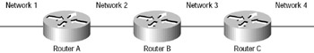
Figure 8.1: Distance-vector operation with three routers.
When distance-vector routers start up or get powered on, they get to know their neighbors; that is, they learn the metrics (hops) to the other routers on each of their interfaces. As the distance-vector network-discovery updates continue (every 30 seconds for IP RIP), routers discover the best path to destination networks. The paths are calculated by and based on the number of hops the routers are from each neighbor. In Figure 8.1, Router C knows Router B is connected to Network 1 by a metric of one. That means it must be a metric of two for Router C to get to Network 1. Router C will never be aware of the whole internetwork—it only knows secondhand what is “gossiped to it.”
Remember convergence? Whenever the network topology changes for any reason, route table updates must occur by each router sending out its entire route table in the form of a broadcast to all the other routers. When a router receives the tables, it compares them to its own table. If it discovers a new network, or what it considers a faster way to get to one, it updates its table accordingly with that information.
Hop Count
What’s the best way to a network? The original distance-vector routing algorithm maintains that “the fewer hops, the better,” and uses only hop counts when making its routing decisions. Take a look at Figure 8.2.
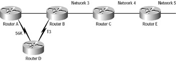
Figure 8.2: Distance-vector network decisions
Router A is getting to Router D through a 56KB WAN link. Router A can also reach Router D via Router B, which can get to Router D through a T3. Which is faster? According to distance-vector routing, the fastest route would be through the 56KB pipe. Imagine sending 500MB files to a server plugged into a hub going to Router D. It would take all day (and night)! So why in the world would it choose that path? Because distance-vector routing uses only metrics (hops) to base its routing decisions on, and in its opinion, one hop is better than two. The solution, of course, is to lie to Router A that the metric to Router D via the 56KB circuit is really three. This can be done manually and will cause Router A to determine that two hops are better than three.
Routing Loops
A problem with distance-vector routing is routing loops. These can occur because every router is not updated at close to the same time. Let’s say that the interface to Network 5 in Figure 8.2 fails. All routers know about Network 5 from Router E. Router A, in its tables, has a path to Network 5 through Routers B, C, and E. When Network 5 fails, Router E tells Router C. This causes Router C to stop routing to Network 5 through Router E. But Routers A, B, and D don’t know about Network 5 yet, so they keep sending out update information. Router C will eventually send out its update and cause Router B to stop routing to Network 5, but Router A and Router D are still not updated. To Router A and Router D, it appears that Network 5 is still available through Router B with a metric of three.
So Router A will send out its regular 30-second “Hello, I’m still here— these are the links I know about” message, which includes reachability for Network 5. Routers B and D then receive the wonderful news that Network 5 can be reached from Router A. So Routers B and D send the information that Network 5 is available. Any packet destined for Network 5 will go to Router A to Router B and then back to Router A. This is a routing loop—what do you do to stop it?
Counting to Infinity
The routing loop problem just described is called counting to infinity, and it’s caused by gossip and wrong information being communicated and propagated throughout the internetwork. Without some form of intervention, each time a packet passes though a router, the hop count increases indefinitely.
One way of solving this problem is to define a maximum hop count. Suppose that a distance-vector routing protocol permits a hop count of up to 15, so anything that requires 16 hops is deemed unreachable. In other words, after a loop of 15 hops, Network 5 will be considered down. This means that counting to infinity, also known as exceeding TTL, will keep packets from going around the loop forever. Though a good solution, it won’t remove the routing loop itself. Packets will still be attracted into the loop, but instead of traveling on it unchecked, they just whirl around for 16 bounces and then die.
Split Horizon
Another solution to the routing loop problem is called split horizon. It reduces incorrect routing information and routing overhead in a distance-vector network by enforcing the rule that information cannot be sent back in the direction from which that information was received. It would have prevented Router A from sending the updated information it received from Router B back to Router B.
Route Poisoning
Another way to avoid problems caused by inconsistent updates is called route poisoning. When Network 5 goes down, Router E initiates route poisoning by entering a table entry for Network 5 as 16 or unreachable (sometimes referred to as infinite). By poisoning its route to Network 5, Router E is not susceptible to incorrect updates about the route to Network 5. Router E will keep this information in its tables until Network 5 comes up again, at which point it will trigger an update to notify its neighbors of the event.
Route poisoning and triggered updates will speed up convergence time, because neighboring routers don’t have to wait 30 seconds (an eternity in computer land) before advertising the poisoned route.
Hold-Downs
And then there are hold-downs. Hold-downs work with triggered updates to prevent regular update messages from reinstating a route that’s gone down. Hold-downs help prevent routes from changing too rapidly by allowing time either for the downed route to come back or for the network to stabilize somewhat before changing to the next best route. Hold-downs also tell routers to restrict, for a specific time period, any changes that might affect recently removed routes. This prevents inoperative routers from being prematurely restored to other routers’ tables.
Hold-downs use triggered updates, which reset the hold-down (HD) timer, to let the neighbor routers know of a change in the network. There are three instances when triggered updates will reset the hold-down timer:
-
The HD timer expires.
-
The router receives a processing task proportional to the number of links in the internetwork.
-
Another update is received indicating the network status has changed.
Link-State Routing
The link-state routing algorithm maintains a more complex table of topology information. Routers using the link-state concept are privileged to a complete understanding and view of all the links of distant routers, plus how they interconnect. The link-state routing process uses link-state packets (LSPs) or Hello packets to inform other routers of distant links. In addition, it uses topological databases, the shortest path first (SPF) algorithm, and of course, a route table.
Network discovery in link-state routing occurs quite differently than it does with distance-vector routing. First, routers exchange Hello packets (LSPs) with one another, giving them a bird’s-eye view of the entire network. In this initial phase, each router communicates only its directly connected links. Second, all routers compile all of the LSPs received from the internetwork and build a topological database. After that, the SPF computes how each network can be reached, finding both the shortest and most efficient paths to each participating link-state network. Each router then creates a tree structure with itself representing the root.
The results are formed into a route table, complete with a listing of the best paths—again, the best paths are not simply the shortest but the most efficient. Once these tasks are completed, the routers can use the table for switching packet traffic.
Our senses can help us determine whether we enjoyed a particular restaurant. Our eyes and ears evaluate the ambiance. Our senses of smell, sight, and taste test the food itself. And we may tangibly examine the linens, utensils, or furnishings. This is a link-state approach.
Unlike distance-vector routing, which is similar to a one-sense evaluation, link-state routing understands that in order for a packet to get from Router A to Router D most efficiently, the shortest path is via the T3—not through the painfully slow 56KB line. It knows this because it doesn’t simply base its path choice decisions on hop count; it also analyzes characteristics like available bandwidth and the amount of load on links to conclude what is truly the best path to a destination.
Convergence
Link-state routers also handle convergence in a completely different manner than distance-vector does. When the topology changes, the router or routers that first become aware of the event either send information to all other routers participating with the link-state algorithm, or they send the news to a specific router that’s designated to consult for table updates.
A router participating in a link-state network must take the following steps in order to converge:
-
Remember its neighbor’s name, when it’s up/down, and the cost of the path to that router.
-
Create an LSP that lists its neighbor’s name and relative costs.
-
Send the newly created LSP to all other routers participating in the link-state network.
-
Receive LSPs from other routers and update its own database.
-
Build a complete map of the internetwork’s topology from all the LSPs received, and then compute the best route to each network destination.
Whenever a router receives an LSP, the router recalculates the best paths and updates the route tables accordingly.
Power, Memory, and Bandwidth Needed
Some issues that must be considered when using link-state routing are processing power, memory usage, and bandwidth requirements.
To run the link-state algorithm, routers must have more power and memory available than what they require to run distance-vector routing. A Cisco router is designed specifically for this purpose.
In link-state routing, routers keep track of all their neighbors and all the networks they can reach. All that information—including various databases, the topology tree, and the route table—must be stored in memory!
Dijkstra’s algorithm states that a processing task proportional to the number of links in the internetwork multiplied by the number of routers in the network will compute the shortest path. What he means is that you need real processing power, ample memory, and a lot of bandwidth. In other words, you’ll make a trip over the Rockies much easier with a V-8, 300-horsepower engine than with 150-horsepower in a four-banger.
Why is the bandwidth requirement so important? Because when a link- state router comes online, it floods the internetwork with LSPs or Hello packets and reduces the bandwidth available for actual data. You remember data, right? That stuff you’re trying to get from point A to B.
The good news is that, unlike distance-vector routers, after this initial network deluge, link-state routers update their neighbors only every two hours on the average—unless a new router comes online or a link drops. And this two-hour period can be changed to be compatible with your bandwidth requirements. Let’s say you have 56KB links to different continents. Would you use RIP (a distance-vector protocol) that updates every 30 seconds, or OSPF (a link-state protocol) that can be configured to update every 12 hours?
Another great thing about link-state routing is that with it, routers can be configured to use a designated router (DR) as the target to consult for all changes. All other routers on the same segment as the DR can contact this router directly for any pertinent network events instead of using the LSP broadcasts to communicate information.
You might be wondering what happens if the routers don’t get an LSP packet? Or what happens if the link is slow and the network topology changes twice before some of the routers even receive the first LSP? Well, link-state routers can implement LSP time stamps, plus they can also use sequence numbers and aging schemes to avoid the spread of inaccurate LSP information. These features would be necessary only in large internetworks.
Comparing Distance-Vector Routing to Link-State Routing
So, as you can see, there are quite a few major differences between distance- vector and link-state routing algorithms. Let’s take a moment to go over a few:
-
Distance-vector routing gets all its topological data from secondhand information or network gossip, whereas link-state routing obtains a complete and accurate view of the internetwork by compiling LSPs.
-
Distance-vector routing determines the best path by counting hops— by metrics. Link-state routing uses bandwidth analysis, plus other pertinent information (better metrics) to calculate the most efficient path.
-
Distance-vector routing updates topology changes in 30-second intervals, adjustable in most cases, which can result in a slow convergence time. Link-state routing can be triggered by topology changes, resulting in faster convergence times as LSPs are passed to other routers, sent to a multicast group of routers, or sent to a specific router.
All things considered, when it comes to routing protocols, there isn’t any one solution for all networks. Routing choices shouldn’t be based solely on speed or cost, because multi-vendor support or standards may well outweigh these factors. Considerations such as network simplicity, the need to set up and manage quickly and easily, or the ability to handle multiprotocols without complex configurations can be pivotal in making proper decisions for your network.
If you’re still unclear on the best approach, how about a compromise? Utilizing the strengths of both, or hybrid routing, can be a great solution.
Balanced Hybrid Routing
Balanced hybrid, or balanced routing, combines and uses the best of both distance-vector and link-state algorithms.
Although the hybrid approach does employ distance vectors with more accurate metric counts than those used by distance-vector routing alone to determine the path to an internetwork, it can converge quickly, thanks to the use of link-state triggers. Additionally, hybrid routing uses a more efficient link-state protocol that helps mitigate the problem of high bandwidth, processor power, and memory needs.
Some examples of hybrid protocols are OSI’s IS-IS (Intermediate System– to–Intermediate System) and Cisco’s EIGRP (Enhanced Interior Gateway Routing Protocol).
Now that we have discussed the differences in routing protocols in general, let’s take a look at some specific routing protocols and how they operate.
|
EAN: 2147483647
Pages: 201