Advanced Fact Table ETL Concepts
The advanced topics in fact table ETL involve changing data grain from the sources to the fact table, handling missing dimension records, and dealing with late-arriving facts.
Managing Fact Table Grain
Many fact table scenarios require data grain changes. This means that the source data coming into the ETL process must be modified to match the record detail in the fact table. For example, you may have a source feed with a certain level of data like product sales at a store for a day. This is called the grain of the data. The fact table destination for the same data coming into the process might be at a different level, such as rolled-up to the week level. In this case, the data grain has changed from day to week. Rolling up data may not always be based on time. For example, a product may be rolled up to a sub-category or category level.
Data Grain Change Scenarios
Grain changes come in many different forms, including some of these common scenarios:
-
Consolidating sources, such as combining multiple tables or files together or joining sources to produce a complete set of business keys needed for the fact table. A common situation is when multiple locations within an organization use different copies of the same system. To report off of a combined fact table, these sources must be consolidated together.
-
Breaking out sources may be required if you have a single table that populates multiple fact tables. For example, an ERP system may export a file that is the transactions for two different fact tables, based on transaction category. In this case, the rows would need to be divided.
-
Roll-up summarizations are a common grain change, where the source feed is at a lower level of detail than the required fact table based on reporting needs. Many situations do not require the detail grain of the source for reporting, which has a side benefit of performance gains and reduced storage requirements.
-
Allocating down or blowing-out the grain is a less common, but interesting, grain change. This is when the level of detail in the fact table is actually a lower grain than what the source system is providing. This may sound impossible, and, in reality, the exact detail cannot be achieved. As an example, an industry data provider may be sending a summarization of sales at a category level, but this detail can be broken down to a sub-category or product level if the percentage breakout is known.
-
Pivot or un-pivot dimensionality takes a source data and converts columns to rows or rows to columns. The most common pivoting needed for fact table data is when the source is coming from a fourth-normal form design, or key-value pair. This data may need to be un-pivoted to de-normalize the data for the fact table match.
Other types of grain changes and scenarios are common, and this transformation requirement (data grain changes) will need to be handled for many fact table ETL processes.
Handling Data Grain Changes with SSIS Transformations
How are these grain changes handled with Integration Services? SSIS includes several built-in transformations to help manage fact table grain changes from the Aggregate transformation to the Pivot. The following table describes several transformations and potential uses to handle different grain changes.
| Transformation | Data Usage |
|---|---|
| Pivot | Converts columns to rows. Useful in a flattened recordset to normalize the grain of a source that will be used for a fact load. |
| Unpivot | Converts rows to columns. Useful for key-value pairs that are common in auditing tables, to collapse rows to columns, and de-normalize the grain. |
| Conditional Split | Allows data routing and filtering. Useful when a source feed needs to be filtered for a fact load, or a single source needs to be split to different fact loads. |
| Aggregate | Summarizes source data. Useful for sources that need to be rolled up to a higher level grain for the fact table load. Can also be used to aggregate across multiple key sets for multiple fact table outputs. |
| Sort | De-duplicates data (and sorts). Provides the ability to remove duplicates across the sort key columns. Useful for sources that need to be pared down based on duplicate records. |
| Union All | Stacks rows of data from multiple sources. Useful when more than one source table or feed matches in structure and is required to be combined for a fact table load. Rows are not joined, but rather passed through. Provides similar semantics to a relational UNION ALL operation. |
| Merge | Combines two identical sources with matching sorted inputs. Similar to the Union All, this transformation can also combine source data for a fact load, especially when the sources are sorted, while preserving the sort order. |
| Merge Join | Joins two sources on a set of keys. Useful when several sources’ entities need to be consolidated for a single fact load. Joins across rows, rather than stacking rows, which allows for columns from both inputs to be included in the output. Also allows the ability to allocate rows to a lower grain by providing multiple output rows across matches. Provides similar semantics to relational JOIN operations (INNER JOIN, LEFT OUTER JOIN, FULL OUTER JOIN). |
| Lookup | Includes Augments columns from a reference table to the output. Useful to also correlate sources, by providing the ability to augment columns from a relational table to the pipeline based on matching source key columns. Can also be used as a filter mechanism to identify matches and non-matches. |
| Derived Column | Allows calculations for allocation with a row. Useful when combined with other transformations. |
| Term Extraction | Provides word-to-text column matching. Useful for text mining–based fact tables to do analysis on words within a source text column. Allocates the grain to the word level of a source. |
| Transformation | Data Usage |
|---|---|
| Term Lookup | Provides English noun-to-text column matching. Similar to the Term Extraction transformation, allocates records down to the word level of a text column, based on an input word list. |
| Script Component | Provides advanced grain-changing capabilities. Useful for many complex scenarios not included in the out-of-the-box capabilities, such as advanced pivoting, filtering, combining, and so on. |
Even beyond what is listed, grain changes can also be achieved by combining these different out-of-the-box transformations together, thus allowing for a fairly comprehensive toolset to handle unique scenarios.
Grain Change SSIS Example
The sales fact tables are a good example of a common grain change from a data source to a fact table destination. In the source AdventureWorks database, the sales transactions are kept in the sales header and sales detail tables. These tables need to be combined together to generate a source record that matches the fact table records. Furthermore, the destination fact tables, Internet sales fact, and reseller sales fact come from the same source, so a separation of the source rows is needed to load these two fact tables separately.
In order to load the fact tables, several steps are involved in the process:
-
The sales header and sales detail records need to be combined to generate all the business keys needed for the load.
-
Records already loaded into the fact tables need to be filtered.
-
The transformed fact records need to be routed to the Internet sales and reseller sales fact tables, respectively.
To demonstrate this, the rest of the sales load package will be shown, picking up where Figure 5-17 left off. At the point in the data flow shown earlier, you are now ready to complete the data flow load. First of all, the dimension lookup and measure calculation discussion earlier in this chapter considers the sales fact table load scenario, which included several dimension lookups and several measures that needed calculations. With the sales fact tables, any record marked as an online order is a direct-to-consumer sale that originated through the Internet. Therefore, these rows must be inserted into the Internet sales fact table. Alternately, any record that is not an online order originates from a reseller transaction and, therefore, should be loaded into the Reseller fact table. Figure 5-28 shows the completed data flow for the sales load package.
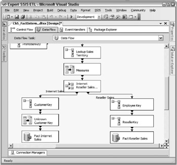
Figure 5-28: Completed data flow for the sales load package
The Conditional Split handles the routing of the fact records to the appropriate fact table. Figure 5-29 shows the Conditional Split editor, which contains the condition OnlineOrderFlag == TRUE.
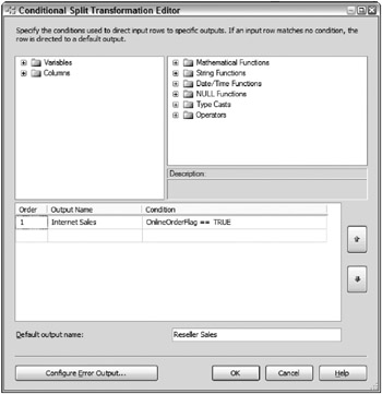
Figure 5-29: Conditional Split editor containing the condition OnlineOrderFlag == TRUE
The rows that meet this criterion are Internet sales orders routed to one output. Every other record is a reseller sale. Therefore, these records are sent out the default output, which is named Reseller Sales.
You will notice that the output of the Conditional Split contains a couple of Lookup transformations on the Internet Reseller Sales output, and one Lookup transformation on the Internet Sales output. This is because the two sales fact tables contain a couple of several different dimension keys. A Customer dimension relationship exists in the Internet Sales fact and a reseller and employee dimension relationship exists in the Reseller Sales fact. Finally, the data flow destinations perform fast loads into the two fact tables, respectively.
Consolidating Source Feeds Example 1
So far, the sales fact table package reviewed in this chapter handled the key lookups and loaded the data into the fact tables. However, this data load package is the second package involved in the sales fact table ETL. The first package that is run for the sales fact is a staging package that consolidates source rows, cleanses data, and filters the records required for the load. Because of the complexity of the data cleansing and correlation, an intermediate staging table was chosen to simplify the ETL and provide a data restartability point.
In the incremental extraction discussion in Chapter 3, Figure 3-32 shows the method used to identify new fact records. In that example, the source records were being pulled from a flat file. But suppose that the source for the sales came from a relational database in two tables, a header and detail, which happens to be the case in the AdventureWorks database. In this scenario, the header and detail tables would need to be combined. Figure 5-30 shows the OLE DB Source adapter editor, which highlights the SQL statement used.
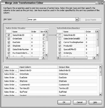
Figure 5-32: Merge Join editor
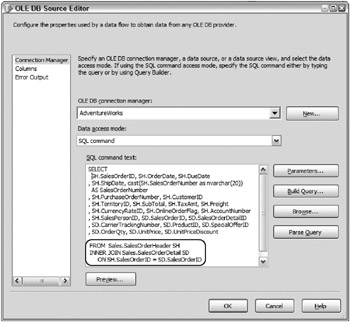
Figure 5-30: OLE DB Source adapter editor
The reason a SQL join was used in this case is because the source system tables are directly related and supported by foreign keys and indexes. The relational database query optimizer efficiently handles the join of the sales header and sales detail tables. However, in the case when the source feed does not come from a database system, or the database cannot optimize the join effectively enough without either straining the source system or slowing down the extraction, then an alternate approach should be taken. Figure 5-31 shows the same extraction package with the sales header and sales detail tables separated into different source adapters.
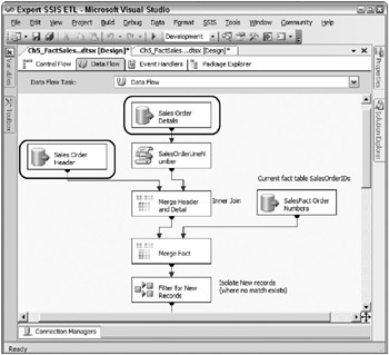
Figure 5-31: Same extraction package with the sales header and sales detail tables separated into different source adapters
To perform the correlation from both source files, a Merge Join transformation is used. Figure 5-32 shows the Merge Join editor. Both source adapters contain SQL statements with explicit ORDER BY operations on the SalesOrderID key, and the adapter is marked as pre-sorted, as described in Chapter 4.
An Inner join is used in the Merge Join transformation, since the source system that created the files uses referential integrity. Therefore, no records will be lost in the join. A Lookup transformation could have been used in this example with the sales header in the Lookup transformation reference table, because the lookup would be across the SalesOrderID and the SalesOrderID, which has a unique constraint as the primary key. However, if your sales header and sales detail tables were coming from files, a Merge Join approach would be required since the Lookup component is unable to directly read in flat file data.
Consolidating Source Feeds Example 2
Do you have a scenario where you are processing multiple identical source files from different company locations? Given one of the goals of data warehousing, which is to bring related data together, a common situation is dealing with multiple feeds from the same application installed in different locations. In other words, you may have several identical files or need to run several identical queries from different installations of the same application.
Briefly, two approaches are possible. The first is to use a ForEach Loop Container to iterate through the files, updating the connections in each loop and running the same data flow multiple times with the updated connections. Chapter 3 discussed a method of looping through files (see Figure 3-10) and updating the connections. Essentially the ForEach Loop Container iterates through the files in a folder, and for every file the connection is updated by a property expression (or alternately a Script Task).
Alternately, a second approach combines the source files in the data flow. In Figure 5-33, three identical files are brought together with a Union All transformation. If your data files are pre-sorted, a Merge transformation would accomplish the same thing, with the benefit of maintaining the sorting downstream.
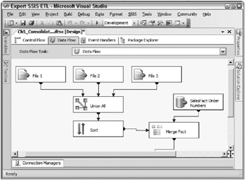
Figure 5-33: Three identical files brought together with a Union All transformation
This approach is useful for smaller files and smaller file counts. The addition of the Sort will add memory overhead, and the file count needs to remain static. However, this approach can be effective when dealing with a contained number of feeds that are very consistent in availability. Otherwise, consider a looping approach.
Handling Missing Dimension Lookups
When the fact table is being loaded and a dimension match is not available, then the fact ETL needs to assign a placeholder surrogate key for the row to be successfully inserted. Dimension foreign keys in the fact table usually do not allow NULL values. Two common approaches exist. Option 1 involves using a generic unknown surrogate key for the missing key. Commonly a surrogate key value of 0, 1, or -1 is reserved for the missing key. Option 2 involves adding a placeholder record in the dimension table with the business key that previously did not exist in the dimension.
Option 1 can be handled through a Derived Column, replacing any NULL values in the surrogate keys with the generic unknown surrogate key. However, this choice will not allow the fact row to ever be updated with the right dimension key, should the dimension source record be available at a later date.
The second option, called an inferred member, offers greater flexibility and will be the focus of this section. In Chapter 4, consideration is given to updating the inferred member dimension record when the missing dimension source is available. This section looks at creating the inferred member during the fact load.
Before looking at how to handle inferred members with SSIS, here’s a quick visual reminder from Chapter 4 about inferred members.
There are at least three ways to handle inferred member creation during the fact-loading process:
-
Create a pre-data flow check of the source rows to see if any missing dimension members exist, and subsequently load them first, before you load the primary data flow for the fact table.
-
Use a post-data flow process. During the primary fact load data flow, only fact source records that have every dimension match immediately available are loaded into the fact table. Any row with at least one missing dimension member is staged to a temporary table. After the primary fact load data flow, the inferred members are added to the dimension table, and then the staged fact source rows are re-processed with complete matches.
-
Use an in-line data flow approach. During the fact row processing, if a missing dimension record exists, add the dimension record mid-stream in the data flow, and bring the new surrogate key back so that all the fact source records can be added to the fact table.
Unfortunately, none of these approaches comes with an Easy Button. Each has its complexities, benefits, and drawbacks. The pre-data flow choice works well when only one or two dimensions require inferred members, and it is okay to scan the source file or table two times (the first to check for inferred members, and the second to load the fact rows). It would involve an initial data flow with dimension Lookups, where any missing lookup records are sent to a dimension destination. The post-data flow requires a few steps: Staging records with missing dimensions, adding the inferred members, and then running the fact load process a second time to associate the newly created inferred member keys and load the rows into the fact table.
The in-line data flow choice comes with some advantages, but requires more complex data flow component configuration. One thing to keep in mind is that, if a dimension record is missing for one fact source row, it is possible that the same dimension record may come across a second time (or more) during the same load. In this common case, the inferred member should be added only once; otherwise duplicates will be generated in the dimension table.
Using out-of-the-box transformations, one data flow approach involves redirecting the missing record, handling the inferred member, and joining back the new record into the data flow. Figure 5-34 shows the sales fact data flow, with inferred member handling of the product dimension.
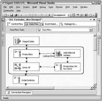
Figure 5-34: Sales fact data flow with inferred member handling of the product dimension
The product dimension lookup is configured as a full cached lookup, and the error output is set to redirect error rows, in the event of a missing record. All error rows are sent out the red path into an OLE DB Command transformation. This component calls a SQL stored procedure, passing in the ProductAlternateKey (or ProductID from the source). The following code shows the details of the TSQL procedure:
CREATE PROCEDURE upCreateProductInferredMember @ProductAlternateKey nvarchar(25) AS IF NOT EXISTS SELECT ProductAlternateKey FROM AdventureWorksDW.dbo.DimProduct WHERE ProductAlternateKey = @ProductAlternateKey) BEGIN INSERT INTO AdventureWorksDW.dbo.DimProduct ( ProductAlternateKey,ProductSubcategoryKey ,EnglishProductName,SpanishProductName ,FrenchProductName,FinishedGoodsFlag ,Color,StartDate,EndDate,Status) VALUES (@ProductAlternateKey ,0,'NA','NA','NA',1,'NA' ,GETDATE(),NULL,'Inf') END Within the stored procedure, the IF NOT EXISTS line checks to see if the business key already exists, in which case, the procedure does not need to re-add it. If the business key does not exist then the procedure adds the inferred member with the business keys and unknowns for attributes.
Because the OLE DB Command cannot receive any returned value, the surrogate key needs to be acquired in a second step. The output of the OLE DB Command is passed to a second Lookup transformation. This Lookup is configured with a disabled cache, as Figure 5-35 highlights. Disabling the cache has the effect of forcing the Lookup component to query the database directly for the required values, instead of utilizing an in-memory cache. A partial-cache could also be used in this context, where the cache is built as new matches are received from the lookup reference table.
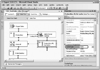
Figure 5-35: Lookup configured with a disabled cache
Every row passed through the OLE DB Command transformation needs the product surrogate key. The Lookup queries the product dimension and returns the right surrogate key. Figure 5-36 shows the Lookup editor Columns tab with the returned surrogate key added as ProductKey_inferred to the data flow.
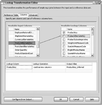
Figure 5-36: Lookup editor Columns tab with the returned surrogate key added
The final step is to bring the fact row back into the main pipeline of records that initially matched the dimension records. This is handled with a Union All transformation. Figure 5-37 shows the Union All editor.
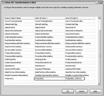
Figure 5-37: Union All editor
Of note, the ProductKey column from the product Lookup is matched with the ProductKey_inferred from the inferred member Lookup, thus giving a complete set of product surrogate keys from the source fact rows that can then be inserted into the fact table destination.
If you have been counting, this model requires three queries against the product dimension table for a new inferred member. The first checks for the record, the second adds the record, and the third gets the surrogate key. Furthermore, every time the same ProductAlternateKey comes through the inferred member process, the product dimension is queried again to check for the record, and again to return the key. When considering that the inferred members should make up a very small minority of source records, this solution may work well and not pose scalability issues. However, a second choice is available that presents a more efficient in-line approach to inferred members.
A Script Component can be used to perform a similar process, but at the same time, increasing the performance by reducing the queries against the dimension table. Rather than describe the solution here, Microsoft has included the code and examples in the Project REAL solution, available for download on the Project REAL site (www.microsoft.com/sql/bi/projectreal), and written up in the Project REAL “ETL Design Practices” paper, also available for download. In brief, the Script component (acting like a transformation) also calls a procedure. However, the procedure returns the surrogate key in the same step and maintains its own cache of ProductAlternateKey with matching surrogate keys in the event the same business key resurfaces.
The bottom line is that choices are available to handle inferred members, and although the processes and code may add complexity to the ETL, the overall benefits are significant for missing dimension handling.
Handling Late-Arriving Facts
Like it sounds, a late-arriving fact is when a fact source row comes through the ETL process at some amount of time after the source row was actually generated. Perhaps a sales record is delayed for a day or so for verification purposes, and then made available to the ETL. The only reason this may require special handling is when a dimension contains Type 2 historical attributes. If the associated record in the dimension table has gone through a Type 2 historical change, then the late-arriving fact row may need to look back to an outdated dimension record for the most accurate dimension association.
One approach for this scenario is to check the current dimension StartDate with the fact transaction date and, if the dimension StartDate is later than the fact transaction date, then send the row out for special handling. Figure 5-38 shows an example of the sales fact load data flow, again focused on the product dimension Lookup.
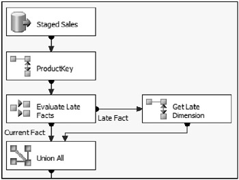
Figure 5-38: Sales fact load data flow focused on the product dimension Lookup
The Lookup for the product dimension returns both the product surrogate key along with the StartDate (aliased as ProductStartDate) of the dimension, since the product dimension contains Type 2 historical attributes. The very next transformation, a Conditional Split, compares the dates. Figure 5-39 shows the Conditional Split editor.
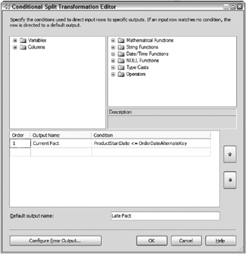
Figure 5-39: Conditional Split editor
If the order date of the sale (OrderDateAlternateKey) is less than or equal to the dimension’s start date, then the surrogate key must be replaced with the correct outdated surrogate key. The rows redirected to the default output called Late Fact are sent into another Lookup transformation, with special configuration to handle the date range. Figure 5-40 shows the Advanced tab of the second Lookup transformation.
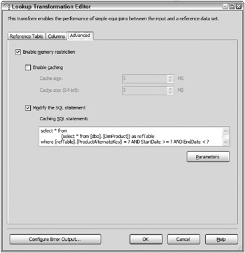
Figure 5-40: Advanced tab of the Lookup transformation
Notice that the Enable memory restriction and Modify the SQL statement check boxes are selected, which allow a custom query to be entered. The query is redefined with parameters to handle the date range. These parameters are mapped to the ProductAlternateKey, the OrderDateAlternateKey, and the same OrderDateAlternateKey again, as Figure 5-41 shows (by clicking the Parameters button).
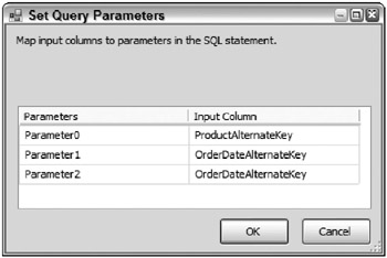
Figure 5-41: Mapped parameters
Using this approach does not allow caching. However, the number of records requiring this handling is usually significantly small. One trick is required to get the modified SQL statement to work. The Column Mappings tab needs to include the OrderDateAlternateKey mapped to a column in the reference table (mapped to StartDate because it made the most sense) so that the lookup can see the OrderDateAlternateKey for parameterization. Without this, the transformation will fail with the error referencing the OrderDateAlternateKey as not existing. Also note, because the SQL statement is being modified, the configured column mapping will not apply, so it is, therefore, okay to map the OrderDateAlternateKey.
Advanced Fact Table Loading
Fact table loading is an important discussion point for scalability and performance. And when dealing with large volumes in the hundreds-of-millions of rows, data flow destination optimization will be a key performance point.
Chapter 12 discusses optimizing destinations for heterogeneous data and bulk loading, respectively. Choosing the right provider and optimizing the settings are reserved for that discussion, including partitioned table data load optimization.
EAN: 2147483647
Pages: 111