Dimension ETL: The Challenge

As already mentioned, dimension ETL often consumes the largest portion of a data warehouse ETL effort. But even beyond the challenges presented of handling history, managing surrogate keys, and accounting for different dimension designs, dimension ETL must manage the source system complexities, and must consolidate them down from the source to the dimension structure in the data warehouse. Figure 4-3 compares the table structures of the product dimension destination in the AdventureWorksDW database with the multiple related product tables from the AdventureWorks database source.

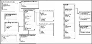
Figure 4-3: Comparison of table structures of the product dimension destination

The left side of the table layout represents the AdventureWorks transactional system, with nine related tables that focus on the product dimension. These tables involve many-to-many relationships and one-to-many primary to foreign key relationships, organized into a transactional third normal form. The challenge for the ETL process is taking the source data and transforming it to a structure that can be compared with the dimension in order to handle dimension history and changes. The challenge is also ensuring that the ETL is scalable and manageable, simple for people to follow when administering it, and flexible to handle changes.

The three tables on the right side of the table layout represent the product dimension organized into a snowflake structure. These tables are considered dimensionally normalized, which is a very different organization than the transactionally normalized tables from the source.

So far, this discussion has looked at the theory of dimension ETL and the challenges presented. As the discussion progresses, another consideration will be the preparation steps required to get your data ready for dimension ETL. Following that, the discussions will shift focus to the core dimension ETL, which requires looking at the built-in support within SSIS, looking at handling advanced dimension forms, and concluding with building your own dimension processing package that scales to your volume.

Preparing Your Source Data for Dimension ETL

Before diving into the details of applying SSIS to handle dimension changes, let’s begin with data preparation.

As you saw with the challenge of dimension ETL, it was quite apparent that, in some situations, the source tables may not match one-to-one with the dimension table. In the case of the product dimension outlined earlier, several source tables must be combined to create a consolidated source recordset that matches the columns within the product dimension. Furthermore, data challenges may also require data cleansing and transformation logic to get the information in a consistent form that relates to the data within the matching dimension table.

With SSIS, several out-of-the-box transformations will become key to your transformation and data-cleansing steps, before even getting to the core of dimension processing. Here are some selective transformations that are very useful for this purpose:

• The Data Conversion transformation is valuable to handle data type conversions, such as conversions between Unicode and non-Unicode data types, numeric and float, or text and numeric.

• The Lookup transformation provides the ability to associate sources without requiring relational joins.

• The Derived Column transformation is especially useful in handling NULL values, performing calculations, or applying date functions.

Figure 4-4 shows several data preparation steps useful in the processing of the Product source data. The first objective is to take the third normal form of transactional system and transform it into a structurally equivalent copy of the dimension table in the data flow pipeline.

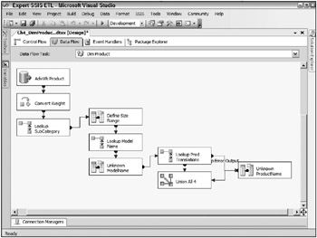
Figure 4-4: Data preparation steps useful in the processing of the product source data

Before you can even use the SCD Wizard, this package requires a series of preparation steps.

The first component is the source adapter, which extracts the source table (Production.Product in this example). Refer to Chapter 3 for a review of the SSIS source adapters. The very next component is a Data Conversion transformation, which changes the data type of the ProductWeight from a Numeric to a Float. This is because the destination table stores this attribute as a float, as opposed to a numeric. Figure 4-5 shows the Data Conversion Transformation Editor. The output column is aliased as Weight to match the column names of the product dimension table.

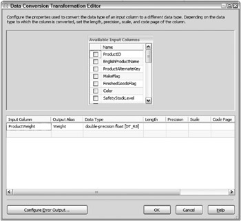
Figure 4-5: Data Conversion transformation

Second, in the product dimension table (which contains the products related to the sale of bicycles and bicycle parts, which AdventureWorks sells), a column exists called SizeRange. This dimension attribute is an example of a dimensional-modeling technique called data banding, where ranges are built from usually numeric sources that have several discrete values, but must be consolidated for grouping. Instead of reporting off of the bicycle sizes one size at a time (38, 40, 42, 43, 45, and so on), there are groupings of the discrete size values, such as 38–40, 42–46, and so on. To handle this requirement, a Derived Column transformation is employed, which considers the size and, based on certain values, how the output is grouped. Figure 4-6 shows the Derived Column transformation used.

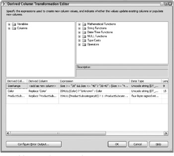
Figure 4-6: Derived Column transformation

The first column in the Derived Column transformation handles the banding by using an SSIS expression-the grammar of which is similar to C-to compare the size to groups of ranges, as shown in the following code. Critical to this expression is the use of an expression-based conditional statement, ≪boolean_expression≫ ? ≪when_true≫ : ≪when_false≫. In this case, the conditional evaluator is recursively embedded to perform multiple comparisons in one statement.

  Size >= "38" && Size <= "40" ? "38-40" :     (Size >= "42" && Size <= "46" ? "42-46" :           (Size >= "48" && Size <= "52" ? "48-52" :                 (Size >= "54" && Size <= "58" ? "54-58" :                       (Size >= "60" && Size < "62" ? "60-62" :                            ISNULL(Size) ? "NA" : Size                       )                 )           )     ) 

In the first condition, if the size for the row being evaluated is 38, then the output range is returned as 38-40. Otherwise, the next condition is checked; and so on, recursively.

The second column used in the example shown in Figure 4-6 deals with unknown values. If there’s a NULL in the Color column, it is trapped and replaced by an Unknown. If the column is not NULL, the actual Color value is used. Note that the third column performs similar NULL-handling for the ProductSubCategory field.

The next transformation in the data flow is an example of data preparation. A Lookup transformation is used to query a second source table that contains an additional attribute needed for the product dimension. Because the Lookup transformation is referencing a source table, the AdventureWorks Connection Manager is selected. In this case, the attribute ModelName comes from a different table in the source. Figure 4-7 shows the Columns tab of the Lookup Transformation Editor.

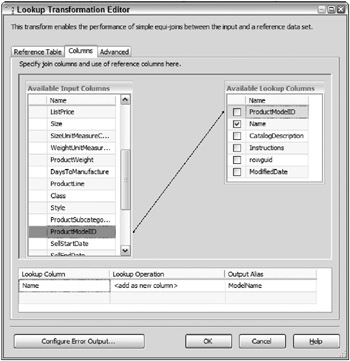
Figure 4-7: Columns tab of the Lookup editor

The available input columns shown on the left come from the Production.Product table that was defined in the source adapter. The available lookup columns on the right come from the Production.ProductModel table, also in the source, which was defined in the Reference Table tab in the same editor.

The lookup is done across the ProductModelID and the Name column is checked, which returns the column into the pipeline column list. The Name column is also aliased as ModelName to match the product dimension table column. In effect, what you have achieved is to take the incoming ProductModelID values and augment them with the corresponding Product Names from a separate table in the source.

The data flow highlighted in Figure 4-4 earlier also shows other transformations used for similar purposes of preparing the data. The output of all these transformations is a pipeline, or a set of columns that align with the dimension table itself. When that preparation process is achieved, then the source data is ready to be matched with the existing dimension data for the handling of dimension changes.

Dimension Change Types

The phrase slowly changing dimension refers to the tracking of dimension changes over time, and, although the phrase is specific to one of the types of tracking, the name has been used to identify the built-in transformation for SSIS.

Important 

Much of dimension change tracking theory (including the slowly changing dimension) was driven by Ralph Kimball of the Kimball Group, Inc. Kimball and the Kimball Group have written extensively on the theory and practicalities of creating dimension models, handling ETL, and planning a data warehouse project. These theories have proven themselves critical to answering the challenge of business intelligence (BI) and data warehousing. In addition to theory, the Kimball Group has produced the Microsoft Data Warehouse Toolkit (Indianapolis: Wiley, 2006), which looks at applying data warehousing theory to the SQL Server 2005 BI technologies.

The question is, as information changes in your dimensions, how do you track those changes? In some situations, data may need to be updated, while other data needs to be tracked historically. Each different tracking requirement is classified as a certain dimension change type. Although there are several different change types, the following are the three most common ones that relate to dimension ETL with SSIS:

• Change Type 0 (fixed)- Also called a fixed attribute, this change type specifies an attribute that should not change over time. An example of this would be gender.

• Change Type 1 (changing)- Oftentimes, tracking the history of changes for a dimension attribute may not provide value. A Type 1 change, also called a changing attribute, is useful when you’re not interested in the previous value of the attribute. For example, if the Color attribute of the product doesn’t provide significant value, then when the color changes, its old value could be overwritten. This technique is also known as Restating History, since, for example, changing the product color from yellow to red would reflect the new color in all previous sales, too.

• Change Type 2 (historical)- A Type 2 change is the slowly changing type in dimension tracking. Also called a historical attribute, this change type is handled by adding a new row. If a customer location changes from New York to Atlanta, rather than overwriting the new location, a second record is created for the customer. Otherwise, if the location is overwritten, the sales history for New York will not include that customer, rather all the sales will appear to have come from Atlanta. This technique is also known as Tracking History, since all changes to dimension attributes can be accurately tracked through time without loss of fidelity.

Two other scenarios are also an important part of an SSIS-based ETL design:

• Creating new members when the data source presents a new record

• Handling missing dimension member processing, called an inferred member

Both of these other dimension processes are supported with SSIS and are discussed in detail later in this chapter.

Change Type 1, a Closer Look

As previously described, a Type 1 or changing attribute requires an in-place update. With this type, you are restating history, and once that update happens, there’s no possibility of querying the older value. Overall, a Type 1 change proves fairly simple to understand and execute. Figure 4-8 shows one record from a source data set that matches a record in a dimension table.

Figure 4-8: Record from a source data set that matches a record in a dimension table

In the reseller source record, the ResellerID matches the ResellerAlternateKey in the reseller dimension. The BusinessType attribute in the reseller dimension is identified as a changing attribute (change Type 1) and the current value is Classic Bikes. The reseller source record, however, indicates that this particular reseller store now is classified as a Specialty Bike Shop. Because the attribute is marked as changing, the value is simply updated. Figure 4-9 shows the updated dimension table record with the new value.

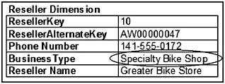
Figure 4-9: Updated dimension table record with the new value

Change Type 2, a Closer Look

A column that is identified as a Type 2 or historical attribute is a little more difficult because it involves adding a row and tracking details of the change. Figure 4-10 shows a record for the product source and the matching record in the product dimension table.

Figure 4-10: Source record for the product dimension, and the matching record in the product dimension table

Notice that two of the attributes, ModelName and Class, are marked as Type 2 historical attributes. In other words, if there is a change, you are interested in keeping the history of the change. In this example, the Class of the product changed from Mid Tier to High Perf. Because a change happened in a Type 2 historical attribute, a new record needs to be added, with a new surrogate key. Figure 4-11 shows the dimension table with the changes applied.

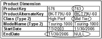
Figure 4-11: Dimension table with the changes applied

The High Perf Class value remains in the original record, but is updated in the new record. Surrogate keys are the lynchpin to handling this, because they allow a new record to be created with the same business key, and all the history in the fact table references the first key, and any new fact records would reference the new surrogate key. This allows someone to run a query to say “show me the sales of the Mid Tier bicycles.” If the change was not tracked historically, the Mid Tier sales would not be available for that bicycle, it would appear as if all the sales for that bicycle were High Perf if querying on Class.

Notice that there are metadata columns to help track the Type 2 historical change-a StartDate and an EndDate. The StartDate for the new record is set to 11/30/2006 and the EndDate is NULL, which indicates the dimension member is the current row. When this new record was added, the EndDate of the original record was updated to the date of that change. The StartDate and EndDate columns provide the capability to know when a dimension member was active, and the capability to identify the current record (that is, when the EndDate is NULL). In this example, there are now two records for this product. However, it is possible to have many different versions of this record.

Another common technique is to use a Boolean column that identifies the current record, which would be marked as True, and the outdated records, which would be marked as False.

Inferred Members

At times, the ETL system may need to handle missing dimension records. When the fact data is being loaded, if the dimension member is not available, the fact row should not just be ignored, but inserted into the fact table with a temporary dimension assignment. An inferred member is a dimension record that has been added during the fact load when the business key from the fact source doesn’t have a match in the dimension table. You might have an inferred member for many reasons:

• If the data in the dimension source or fact source is dirty and the match is not available, then the dimension member may not be available or found in the dimension table.

• Depending on source system requirements, if the dimension source cannot be extracted as often or before the fact table source is extracted and processed, a missing dimension record may occur.

• If the dimension source is not updated as often as the fact source, it may result in missing dimension records during the fact load.

Having missing dimension members is a problem known as an inferred member, but is also commonly called a late-arriving dimension scenario.

For example, at some retailers, products may go on the shelf at a store to be sold before the master product table is updated at a corporate office. Store managers are often given autonomy to sell extra products in their stores outside of the corporate product list. Therefore, data may not enter into the centralized item inventory until later, but the sale is still recorded, causing a late arriving dimension scenario.

When dealing with inferred members, there are really two aspects of the ETL:

• Inserting the inferred member during the fact load

• Updating the inferred member during the dimension load

Adding Inferred Members During the Fact Load

The SSIS mechanisms for this aspect of inferred members is discussed in Chapter 5, but here are some of the basics of what must happen during the ETL. During the fact load, if a dimension record is not available, a placeholder record is added to the dimension table. If you get a business key for a product, but the product doesn’t exist in the dimension table, instead of using a generic unknown that is not associated with any business key, you can add an unknown specific to the business key for the missing record. Later, if or when the dimension record comes in from the source, you can update it with all the attributes. Inferred members are the most complicated part of dimension processing.

Figure 4-12 shows a transactional source for a sales type fact table on the left, and a couple rows from a related dimension table on the right. The source contains a ProductID. However, there’s no match in the dimension table itself. The ProductID (business key) BK-8006F sold for $439.99, but a matching dimension record is not in the dimension table.

Figure 4-12: Transactional source for a sales type fact table (left) and rows from a related dimension table (right)

Handling this as an inferred member, you must add a record to the dimension table during this fact load. What you don’t have are values for all the other attributes of the dimension, which must be set to an unknown value. Figure 4-13 shows the resulting dimension table after the load.

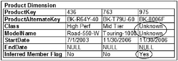
Figure 4-13: Resulting dimension table after the load

Notice that the inferred member has been added with a new surrogate key, but the attributes in the dimension are set to Unknown. Furthermore, there’s another column in the dimension table called the Inferred Member Flag column. This should be set to Yes (or True), because the dimension process needs to know this is an inferred member created during the fact load. That will impact how dimension processing handles that ETL.

Updating the Inferred Member During the Dimension Load

As just discussed, when you’re loading the fact table, if there’s a missing record, you add the record to the dimension table as an inferred member. When you process the dimension table later, if the dimension source becomes available for an inferred member, it can be updated with the missing dimension attributes. It works by essentially updating all the columns for that table. Every attribute becomes like a Type 1 changing attribute, even the Type 2 historical attributes. In other words, instead of creating a new record with the changes, the original record is updated. Figure 4-14 shows one row in the data source for a dimension (on the left), and a few rows from the dimension table. The source contains details for a record that currently exists in the dimension table as an inferred member.

Figure 4-14: Row in the data source for a dimension (left) and rows from the dimension table

If the matching record table in the dimension was added during a normal dimension load, the change in the Class or ModelName column (because they are Type 2 historical) would cause a new record to be generated. However, because the dimension member is marked as an inferred member, instead, every attribute is updated to the new values. Figure 4-15 shows the now updated dimension table.

Figure 4-15: Updated dimension table

Not only are all the attributes updated with the new value, but also the Inferred Member Flag column is marked as No (or false), because you now have the full details of that dimension member. An inferred member turns all the attributes into Type 1 changing until the dimension member details come in from the source.

Important 

You may have a scenario where you want the dimension table to act like an inferred member, even though the dimension is added from the dimension source. If you have a dimension source record that goes through lots of column value changes until at some point the record is stable, consider treating that dimension record as an inferred member until it stabilizes. The drawback in handling the dimension record like a normal dimension with Type 1 changing and Type 2 historical attributes is that every change to a Type 2 historical attribute causes a new record. Waiting until the stabilization will reduce the number of dimension records and, therefore, avoid too much confusion with so many records for a single member.