Changing Summary Calculations

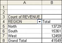
When creating your pivot table report, the PivotTable Wizard will, by default, summarize your data by either counting or summing the items. Instead of Sum or Count, you might want to choose functions such as Min, Max, and Count Numeric. In all, 11 options are available. However, the common reason to change a summary calculation is because Excel incorrectly chose to count instead of sum your data.

One Blank Cell Causes a Count

If all the cells in a column contain numeric data, Excel will choose to sum. If just one cell is either blank or contains text, Excel will choose to count. Be vigilant while dropping fields into the data section of the pivot table. If a calculation appears to be dramatically too low, check to see if the field name reads "Count of Revenue" instead of "Sum of Revenue." When you created the pivot table in Figure 3.6, you should have noticed that your company only had $41,549 in revenue instead of $800 million. This should be your first clue to notice that the heading in A3 reads "Count of Revenue" instead of "Sum of Revenue." In fact, 41,549 is the number of records in the dataset.

Figure 3.6. Your revenue numbers look anemic. Notice in cell A3 that Excel chose to count instead of sum the revenue. This often happens if you inadvertently have one blank cell in your Revenue column.

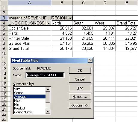
You can easily override the incorrect Count calculation. Activate the PivotTable Field dialog box by double-clicking on Count of Revenue and then change the Summarize By setting from Count to Sum.

Using Functions Other Than Count or Sum

Excel offers a total of 11 functions in the Summarize By section of the PivotTable Field dialog box. The options available are as follows:

• Sum Provides a total of all numeric data.

• Count Counts all cells, including numeric, text, and error cells. This is equivalent to the Excel function =COUNTA().

• Average Provides an average. Figure 3.7 shows a report detailing average sales per region and line of business. An analyst might wonder why the average copier sale in the South is $7,000 higher than in the West.

  Figure 3.7. Average sales per region and line of business.

  

  
  

• Max Shows the largest value.

• Min Shows the smallest value.

• Product Multiplies all the cells together. For example, if your dataset had cells with values of 3, 4, and 5, the product would be 60.

• Count Nums Counts only the numeric cells. This is equivalent to the Excel function =COUNT().

• StdDev and StdDevP Calculates the standard deviation. Use StdDevP if your dataset contains the complete population. Use StdDev if your dataset contains a sample of the population. Figure 3.8 shows the results of two tests. Although the students averaged 87% on both tests, the math test had a higher standard deviation. Standard deviations explain how tightly results are grouped around the mean.

  Figure 3.8. A low standard deviation on the science test means that all the students understand the concepts equally well. A higher standard deviation on the math test indicates that student scores were spread over a wider range.

  

  
  

• Var and VarP Calculates the statistical variance. Use VarP if your data contains a complete population. If your data contains only a sampling of the complete population, use Var to estimate the variance.