Task Two: Filling in Missing Labels When the order-processing system produces a summary report, it enters a label in a column only the first time that label appears. Leaving out duplicate labels is one way to make a report easier for a human being to read, but for the computer to sort and summarize the data properly, you need to fill in the missing labels. 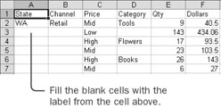 You might assume that you need to write a complex macro to examine each cell and determine whether it's empty, and if so, what value it needs. In fact, you can use Excel's built-in capabilities to do most of the work for you. Because this part of the project introduces some powerful worksheet features, you'll go through the steps before recording the macro. Select Only the Blank Cells Look at the places where you want to fill in missing labels. What value do you want in each empty cell? You want each empty cell to contain the value from the first nonempty cell above it. In fact, if you were to select each empty cell in turn and put into it a formula pointing at the cell immediately above it, you would have the result you want. The range of empty cells is an irregular shape, however, which makes the prospect of filling all the cells with a formula daunting. Fortunately, Excel has a built-in tool for selecting an irregular range of blank cells. -
In a copy of the Nov2002 worksheet in the Chapter02 workbook, select cell A1. -
Choose the Edit menu, and click the Go To command. The Go To dialog box appears. | Tip | You also can press Ctrl+Shift+* to select the current region. Press and hold the Ctrl key while pressing * on the numeric keypad or Shift+8 on the regular keyboard. | -
In the Go To dialog box, click Special. 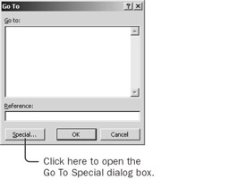 -
In the Go To Special dialog box, click the Current Region option and then click OK. 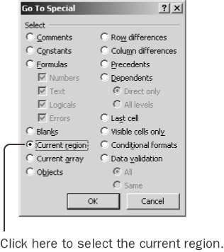 Excel selects the current region-the rectangle of cells including the active cell that is surrounded by blank cells or worksheet borders. -
Choose the Edit menu, click Go To, and then click Special. -
In the Go To Special dialog box, click the Blanks option, and then click OK. Excel subselects only the blank cells from the selection. These are the cells that need new values. 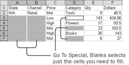 Excel's built-in Go To Special feature can save you-and your macro-a lot of work. Fill the Selection with Values You now want to fill each of the selected cells with a formula that points at the cell above. Normally when you enter a formula, Excel puts the formula into only the active cell. You can, however, if you ask politely, have Excel put a formula into all the selected cells at once. -
With the blank cells selected and D3 as the active cell, type an equal sign (=) and then press the Up Arrow key to point at cell D2. The cell reference D2-when found in cell D3-actually means 'one cell above me in the same column.' -
Press Ctrl+Enter to fill the formula into all the currently selected cells. When more than one cell is selected, if you type a formula and press Ctrl+Enter, the formula is copied into all the cells of the selection. (If you press the Enter key without pressing and holding the Ctrl key, the formula goes into only the one active cell.) Each cell with the new formula points to the cell above it. 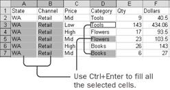 -
Press Ctrl+Shift+* to select the current region. -
Choose the Edit menu, and click Copy. Then choose the Edit menu, click Paste Special, click the Values option, and then click OK. -
Press the Esc key to get out of copy mode, and then select cell A1. Now the block of cells contains all the missing-label cells as values, so the contents won't change if you happen to re-sort the summary data. In the next section, you'll select a different copy of the imported worksheet and follow the same steps, but with the macro recorder turned on. Record Filling the Missing Values -
Select a copy of the Nov2002 worksheet (one that doesn't have the labels filled in), or run the ImportFile macro again. Record Macro  -
Click the Record Macro button, type FillLabels as the name of the macro, and then click OK. -
Select cell A1 (even if it's already selected), press Ctrl+Shift+*, choose the Edit menu, click Go To, click the Special button, click the Blanks option, and then click OK. -
Type =, press the Up Arrow key, and press Ctrl+Enter. -
Press Ctrl+Shift+*. -
Choose the Edit menu, and click Copy. Next choose the Edit menu, click Paste Special, click the Values option, and then click OK. -
Press the Esc key to get out of copy mode, and then select cell A1. Stop Recording  -
Click the Stop Recording button, and save the Chapter02 workbook. You've finished creating the FillLabels macro. Read it while you step through the macro. Watch the FillLabels Macro Run -
Select another copy of the imported worksheet, or run the ImportFile macro again. Run Macro  -
Click the Run Macro button, select the FillLabels macro, and click Step Into. The Visual Basic window appears, with the header statement of the macro highlighted. -
Press F8 to move to the first statement in the body of the macro: Range("A1").Select This statement selects cell A1. It doesn't matter how you got to cell A1-whether you clicked the cell, pressed Ctrl+Home, or pressed various arrow keys-because the macro recorder always records just the result of the selection process. -
Press F8 to select cell A1 and highlight the next statement: Selection.CurrentRegion.Select This statement selects the current region of the original selection. -
Press F8 to select the current region and move to the next statement: Selection.SpecialCells(xlCellTypeBlanks).Select This statement selects the blank special cells of the original selection. (The word SpecialCells refers to cells you selected using the Go To Special dialog box.) -
Press F8 to select just the blank cells and move to the next statement: Selection.FormulaR1C1 = "=R[-1]C" This statement assigns =R[-1]C as the formula for the entire selection. When you entered the formula, the formula you saw was =C2, not =R[-1]C. The formula =C2 really means 'get the value from the cell just above me,' but only if the active cell happens to be cell C3. The formula =R[ 1]C also means 'get the value from the cell just above me,' but without regard for which cell is active. | Tip | For more information about R1C1 notation, type R1C1 references into the Ask A Question box in the Excel window. | You could change this statement to Selection.Formula = "=C2" and the macro would work exactly the same-provided that the order file you use when you run the macro is identical to the order file you used when you recorded the macro and that the active cell happens to be cell C3 when the macro runs. If the command that selects blanks produces a different active cell, however, the revised macro will fail. The macro recorder uses R1C1 notation so that your macro will always work correctly. -
Press F5 to execute the remaining statements in the macro: Selection.CurrentRegion.Select Selection.Copy Selection.PasteSpecial Paste:=xlPasteValues, _ Operation:=xlNone, SkipBlanks:=False, Transpose:=False Application.CutCopyMode = False Range("A1").Select These statements select the current region, convert the formulas to values, cancel copy mode, and select cell A1. You've completed the macro for the second task of your month-end project. Now you can start a new macro to carry out the next task-adding dates. |