Transformations inside the Oracle Server

5.5 Transformations inside the Oracle Server

Section 5.3 introduced transformations and discussed choosing the optimal place to perform the transformations. We've seen examples of transforming the data while loading it using both SQL*Loader and external tables. This section will discuss performing transformations inside the Oracle Server. If you are doing transformations in the Oracle data warehouse, you typically load data into temporary staging tables, transform the data, and then move this data to the warehouse detail fact tables.

When using transportable tablespaces, as discussed in the previous section, the data was moved from the OLTP system to the staging area in the Oracle warehouse. Data that was loaded using external tables or SQL*Loader can be further transformed in a staging area inside the Oracle Server. Oracle 9i provides tools that can be used to implement transformations in SQL, PL/SQL, or Java stored procedures.

In this section we will first look at the SQL to perform the following simple transformations:

• Remove the "-" from product ID and increase the shipping charges by 10 percent.

• Check for invalid product_id's.

• Look up the warehouse key, and substitute it for the PRODUCT_ID.

Then, we will rewrite the first transformation as a table function.

5.5.1 Transformations that cleanse data and derive new data

The SQL UPDATE statement using built-in functions can be used to perform some simple transformations. Continuing with our example, the APR_ORDERS table must be cleansed. Some of the PRODUCT_ID'S contain a "-", which needs to be removed. The fuel costs have increased, so we must add 10 percent to the shipping charges. Both of these operations can be done in one step using the UPDATE statement. A few of the rows are shown before they are transformed.

 SQL> SELECT * FROM apr_orders; PRODUCT TIME_KEY  CUSTOMER  PURCHASE PURCH PURCH SHIP    TODAYS_ ID                ID        DATE     TIME  PRICE CHARGE  SPECIAL ------- --------- --------- -------- ----- ----- ------ ------- SP1001   02-APR-02 AB123457 02-APR-02 1024 28.01 5.45    N SP-1000  01-APR-02 AB123456 01-APR-02 1001 67.23 5.45    N SP-1000  01-APR-02 AB123457 01-APR-02 1002 67.23 5.45    N 

The SQL multiplication operator, (*), will be used to update the shipping charge, and the REPLACE function will be used to replace the hyphen, "-", with an empty quote, "", thus removing it. The modified fields are shown in bold type. The shipping charge has increased from $5.45 to $6. The hyphen has been removed from the PRODUCT_ID.

 SQL> UPDATE apr_orders SET shipping_charge = (shipping_charge + shipping_charge *.10), product_id=REPLACE(product_id, '-',''); PRODUCT TIME_KEY  CUSTOMER  PURCHASE PURCH PURCH SHIP   TODAYS_ ID                ID        DATE     TIME  PRICE CHARGE SPECIAL ------- --------- --------- -------- ----- ----- ------ ------- SP1001  02-APR-02 AB123457 02-APR-02 1024 28.01  6      N SP1000  01-APR-02 AB123456 01-APR-02 1001 67.23  6      N SP1000  01-APR-02 AB123457 01-APR-02 1002 67.23  6      N 

5.5.2 Validating data using a dimension

Often the incoming data must be validated using information that is in the dimension tables. While this is not actually a transformation, it is discussed here, since it is often done at this stage prior to loading the warehouse tables. In our example, we want to ensure that all the PRODUCT_ID'S for the April orders are valid. The PRODUCT_ID for each order must match a PRODUCT_ID in the product dimension.

This query shows that the April data has an invalid PRODUCT_ID, where there is no matching PRODUCT_CODE in the product dimension. Any data that is invalid should be corrected prior to loading it from the staging area into the warehouse.

 SQL> SELECT DISTINCT product_id FROM apr_orders WHERE product_id NOT IN (SELECT product_id FROM product); PRODUCT_ID ---------- SP1036 

5.5.3 Looking up the warehouse key

Now that we have cleansed the PRODUCT_ID column, we will modify it to use the warehouse key. For the next example, a product_code has been added to the product table that will be used to look up the PRODUCT_ID, which is the surrogate key for the warehouse. Figure 5.4, showed theuse of surrogate keys in the warehouse. A portion of the product dimension is displayed.

 SQL> SELECT PRODUCT_ID, PRODUCT_CODE FROM PRODUCT; PRODUCT_ID PRODUCT_CODE ---------- --------          1 SP1000          2 SP1001          3 SP1010          4 SP1011          5 SP1012 

In this next transform we are going to use the PRODUCT_ID in the APR_ORDERS table to look up the warehouse key from the product dimension. The PRODUCT_ID column in the apr_orders table will be replaced with the warehouse key.

 SQL> SELECT * FROM APR_ORDERS; PRODUCT TIME_KEY  CUSTOMER  PURCHASE PURCH PURCH SHIP   TODAYS_ ID                ID        DATE     TIME  PRICE CHARGE SPECIAL ------- --------- --------- -------- ----- ----- ------ ------- SP1001 01-APR-02 AB123456   01-APR-02 24   28.01    6    Y SP1001 01-APR-02 AB123457   01-APR-02 1024 28.01    6    Y SP1061 01-APR-02 AB123456   01-APR-02   24 28.01    8.42 Y SP1062 01-APR-02 AB123457   01-APR-02 1024 28.01    3.58 Y SQL> UPDATE APR_ORDERS A SET A.PRODUCT_ID = (SELECT P.PRODUCT_ID FROM PRODUCT P WHERE A.PRODUCT_ID = P.PRODUCT_CODE); 4 rows updated. 

Note that the original PRODUCT_ID's have been replaced with the warehouse key.

 SQL> SELECT * FROM APR_ORDERS; PRODUCT TIME_KEY  CUSTOMER  PURCHASE PURCH PURCH SHIP   TODAYS_ ID                ID        DATE     TIME  PRICE CHARGE SPECIAL ------- --------- --------- -------- ----- ----- ------ ------- 2      01-APR-02 AB123456   01-APR-02 24   28.01    6    Y 2      01-APR-02 AB123457   01-APR-02 1024 28.01    6    Y 54     01-APR-02 AB123456   01-APR-02   24 28.01    8.42 Y 55     01-APR-02 AB123457   01-APR-02 1024 28.01    3.58 Y 

5.5.4 Table functions

The results of one transformation are often stored in a database table. This table is then used as input to the next transformation. The process of transforming and storing intermediate results, which are used as input to the next transformation, is repeated for each transformation in the sequence.

The drawback to this technique is performance. The goal is to perform all transformations so that each record is read, transformed, and updated only once. Of course, there are times where this may not be possible, and the data must be passed through multiple times.

A table function is a function whose input is a set of rows and whose output is a set of rows, which could be a table-hence the name table function. The sets of rows can be processed in parallel, and the results of one function can be pipelined to the next before the transformation has been completed on all the rows in the set, eliminating the need to pass through the data multiple times.

Table functions use Oracle's object technology and user-defined data types. First, new data types must be defined for the input record and output table. In the following example, the PURCHASES_RECORD data type is defined to describe the records in the PURCHASES table.

 SQL> CREATE TYPE purchases_record as OBJECT (product_id                   VARCHAR2(8), time_key                      DATE, customer_id                   VARCHAR2(10), purchase_date                 DATE, purchase_time                 NUMBER(4,0), purchase_price                NUMBER(6,2), shipping_charge               NUMBER(5,2), today_special_offer           VARCHAR2(1)); 

Next, the PURCHASES_TABLE data type is defined. It contains a collection of PURCHASES_RECORDs, which will be returned as output from the function.

 SQL> CREATE TYPE purchases_table AS TABLE of purchases_record; 

Next, define a type for a cursor variable, which will be used to pass a set of rows as input to the table function. Cursor variables are pointers, which hold the address of some item instead of the item itself. In PL/SQL, a pointer is created using the data type of REF. Therefore, a cursor variable has the data type of REF CURSOR. To create cursor variables, you first define a REF CURSOR type.

 CREATE PACKAGE cur_pack AS TYPE ref_cur_type IS REF CURSOR; END cur_pack; 

Here is our table function , TRANSFORM, which performs the search and replace, removing the hyphen from the PRODUCT_ID and increasing the shipping charge. There are some things that differentiate it from other functions. The function uses PIPELINED in its definition and PIPE ROW in the body. This causes the function to return each row as it is completed, instead of waiting until all rows are processed. The input to the function is a cursor variable, INPUTRECS, which is of type REF_CUR_TYPE defined previously. The output of the function is a table of purchase records of type PURCHASES_TABLE defined previously. The REF CURSOR, INPUTRECS, is used to fetch the input rows, the transformation is performed, and the results for each row are piped out. The function ends with a RETURN statement, which does not specify any return value.

 CREATE OR REPLACE FUNCTION transform (inputrecs IN cur_pack.ref_cur_type) RETURN purchases_table PIPELINED IS   product_id                      VARCHAR2(8);   time_key                        DATE;   customer_id                     VARCHAR2(10);   purchase_date                   DATE;   purchase_time                   NUMBER(4,0);   purchase_price                  NUMBER(6,2);   shipping_charge                 NUMBER(5,2);   today_special_offer             VARCHAR2(1); BEGIN LOOP FETCH inputrecs INTO product_id,       time_key,customer_id,purchase_date,purchase_time,       purchase_price,shipping_charge,today_special_offer;       EXIT WHEN INPUTRECS%NOTFOUND;       product_id := REPLACE(product_id, '-','');       shipping_charge :=(shipping_charge+shipping_charge*.10);       PIPE ROW(purchases_record(product_id,             time_key,             customer_id,             purchase_date,             purchase_time,             purchase_price,             shipping_charge,             today_special_offer)); END LOOP; CLOSE inputrecs; RETURN; END; 

We've rolled back the changes from the previous transforms and are going to do them again using the table function. Here are the data prior to being transformed.

 SQL> SELECT * FROM APR_ORDERS; PRODUCT TIME_KEY  CUSTOMER  PURCHASE PURCH PURCH SHIP   TODAYS_ ID                ID        DATE     TIME  PRICE CHARGE SPECIAL ------- --------- --------- -------- ----- ----- ------ ------- SP-1001 01-APR-02 AB123456   01-APR-02   24 28.01   5.45  Y SP-1001 01-APR-02 AB123457   01-APR-02 1024 28.01   5.45  Y SP1061  01-APR-02 AB123456   01-APR-02   24 28.01   8.42  Y SP1062  01-APR-02 AB123457   01-APR-02 1024 28.01   3.58  Y 

To invoke the function, use it as part of a SELECT statement. The TABLE keyword is used before the function name in the FROM clause. The changes are shown in bold in the following code:

 SQL> SELECT * FROM      TABLE(transform(CURSOR(SELECT * FROM apr_orders))); PRODUCT TIME_KEY  CUSTOMER  PURCHASE PURCH PURCH SHIP   TODAYS_ ID                ID        DATE     TIME  PRICE CHARGE SPECIAL ------- --------- --------- -------- ----- ----- ------ ------- SP1001  01-APR-02 AB123456  01-APR-02   24 28.01    6       Y SP1001  01-APR-02 AB123457  01-APR-02 1024 28.01    6       Y SP1061  01-APR-02 AB123456  01-APR-02   24 28.01    9.26    Y SP1062  01-APR-02 AB123457  01-APR-02 1024 28.01    3.94    Y 

If we needed to save the data, the following code creates a table to save the results of the table function.

 SQL> CREATE TABLE TEST AS SELECT * FROM TABLE(transform(CURSOR(SELECT * FROM apr_orders))); Table created. 

5.5.5 Transformations that split one data source into multiple targets

Sometimes transformations involve splitting a data source into multiple targets, as illustrated in Figure 5.15. A new feature introduced in Oracle 9i, multitable INSERT, facilitates this type of transformation.

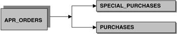
Figure 5.15: Multitable insert.

In the following example, the APR_ORDERS will be split into two tables. All orders that took advantage of today's special offer will be written to the SPECIAL_PURCHASES table. All regular sales will be written to the PURCHASES table. This information could be used to target future advertising. A new table, SPECIAL_PURCHASES, has been created with the same columns as the APR_ORDERS and PURCHASES tables.

The insert statement specifies a condition, which is evaluated to determine into which table each row should be inserted. In this example there is only one WHEN clause, but you can have multiple WHEN clauses if there are multiple conditions to evaluate. If no WHEN clause evaluates to true, the ELSE clause is executed.

By specifying FIRST, Oracle stops evaluating the WHEN clause when the first condition is met. Alternatively, if ALL is specified, all conditions will be checked for each row. ALL is useful when the same row is stored in multiple tables.

 SQL> INSERT FIRST WHEN today_special_offer = 'Y'      THEN INTO special_purchases      ELSE INTO purchases      SELECT * FROM apr_orders; 15004 rows created. 

The four rows with today_special_offer = 'Y', have been inserted into the SPECIAL_PURCHASES table. The remaining rows have been inserted into the PURCHASES table.

 SQL> SELECT COUNT(*) FROM purchases;   COUNT(*) ----------     15000 SQL> SELECT COUNT(*) FROM special_purchases;    COUNT(*) ----------       4 

From the following queries, we can see that the data has been split between the two tables. Purchases made with the value of N in TODAY_SPECIAL_OFFER are stored in the PURCHASES table. Those with the value of Y are stored in the SPECIAL_PURCHASES table.

 SQL> SELECT DISTINCT(today_special_offer) FROM purchases; Today_special_offer ------------------- N SQL> SELECT DISTINCT(today_special_offer) FROM special_purchases; Today_special_offer ------------------- Y 

5.5.6 Moving data from a staging table into the fact table

Once the data has been transformed, it is ready to be moved to the warehouse tables. In Figure 5.14, the April purchases were moved into temporary staging tables in the warehouse. Once the data has been cleansed and transformed, it is ready to be moved into the purchases fact table, as shown in Figure 5.16.

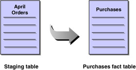
Figure 5.16: Data is moved from a staging table into the fact table.

When the fact table is partitioned, new tablespaces are created for the data file and indexes, a new partition is added to the fact table, and the data is moved into the new partition. The steps are illustrated using the EASYDW example.

Step 1: Create a new tablespace for the April purchases and the April purchases index

Since the purchases table is partitioned by month, a new tablespace will be created to store the April purchases. Another tablespace is created for the indexes.

 SQL> CREATE TABLESPACE purchases_apr2002      DATAFILE 'c:\ora9ir2\oradata\orcl\purchasesapr2002.f'      SIZE 5M      REUSE AUTOEXTEND ON      DEFAULT STORAGE      (INITIAL 64K NEXT 64K PCTINCREASE 0 MAXEXTENTS UNLIMITED) SQL> CREATE TABLESPACE purchases_apr2002_idx      DATAFILE 'C:\ora9ir2\oradata\orcl\PURCHASESAPR2002_IDX.f'      SIZE 3M REUSE      AUTOEXTEND ON      DEFAULT STORAGE      (INITIAL 16K NEXT 16K PCTINCREASE 0 MAXEXTENTS UNLIMITED) 

Step 2: Add a partition to the purchases table

The PURCHASES table is altered, and the purchases_apr2002 partition is added.

 SQL>ALTER TABLE easydw.purchases ADD PARTITION purchases_apr2002 VALUES LESS THAN (TO_DATE('30-04-2002', 'DD-MM-YYYY')) PCTFREE 0 PCTUSED 99 STORAGE (INITIAL 64K NEXT 164 PCTINCREASE 0) TABLESPACE purchases_apr2002; 

Figure 5.17 shows the new partition that has been added to the PURCHASES table and the corresponding PURCHASE_PRODUCT_INDEX.

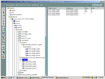
Figure 5.17: Viewing a table's partitions using enterprise manager.

Step 3: Move the table into the new partition

There are a variety of ways to move the data from one table to another in the same database:

• Exchange partition (when the fact table is partitioned)

• Direct path insert

• CREATE TABLE AS SELECT

Moving data using exchange partition

The ALTER TABLE EXCHANGE PARTITION clause is generally the fastest way to move the data of a nonpartitioned table into a partition of a partitioned table. This clause can be used to move both the data and local indexes from a staging table into a partitioned fact table. The reason it is so fast is because the data is not actually moved; instead, the metadata is updated to reflect the changes.

If the data has not previously been cleansed, it can be validated to ensure that it meets the partitioning criteria, or this step can be skipped using the WITHOUT VALIDATION clause. Figure 5.18 shows moving the data from the APR_ORDERS staging table into the PURCHASES fact table using exchange partition.

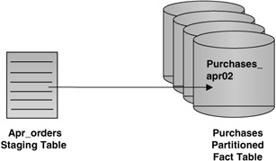
Figure 5.18: Exchange partition.

The following example shows moving the data from the APR_ORDERS into the PURCHASES_APR2002 partition of the EASYDW.PURCHASES table.

 SQL> ALTER TABLE easydw.purchases EXCHANGE PARTITION purchases_ apr2002 WITH TABLE apr_orders WITHOUT VALIDATION; 

After exchanging the partition, there are no rows left in the APR_ORDERS table, and it can be dropped.

 SQL> SELECT * FROM apr_orders; no rows selected SQL> DROP TABLE apr_orders; Table dropped. 

Moving data between tables using direct path insert

If the fact table is not partitioned, you can add more data to it by using direct path insert. A direct path insert enhances performance during insert operations by formatting and writing data directly into the data files without using the buffer cache. This functionality is similar to SQL*Loader direct path mode.

Direct path insert appends the inserted data after existing data in a table; free space within the existing table is not reused when executing direct path operations. Data can be inserted into partitioned or nonpartitioned tables, either in parallel or serially. Direct path INSERT updates the indexes of the table.

In the EASYDW database, since the purchases table already exists and is partitioned by month, we could use the direct path insert to move the data into the table. Direct path insert is executed when you include the APPEND hint and are using the SELECT syntax of the INSERT statement.

 SQL>INSERT /*+ APPEND */ INTO easydw.purchases           SELECT * FROM apr_orders 

In our example, the purchases fact table already existed, and new data was added into a separate partition.

Hint: 

Be sure you have disabled all references constraints before executing the direct load insert. If you do not, the APPEND hint will be ignored, no warnings will be issued, and a conventional insert will be used. Plus, the insert will take a long time if there is a lot of data.

Hint: 

Conventional path is used when using the INSERT... with the VALUES clause, even if you use the APPEND hint.

Creating a new table using CREATE TABLE AS SELECT

If the detail fact table does not yet exist, you can create a new table selecting a subset of one or more tables using the CREATE TABLE AS SELECT statement. The table creation can be done in parallel. You can also disable logging of redo. In the following example, TEMP_PRODUCTS is the name of the staging table. After performing the transformations and data cleansing, the products table is created by copying the data from TEMP_PRODUCTS table.

 SQL> CREATE TABLE products PARALLEL NOLOGGING AS            SELECT * FROM temp_products;