Loading the warehouse

5.4 Loading the warehouse

When loading the warehouse, the dimension tables are generally loaded first. The dimension tables contain the surrogate keys or other descriptive information needed by the fact tables. When loading the fact tables, information is looked up from the dimension tables and added to the columns in the fact table.

When loading the dimension table, you need both to add new rows and make changes to existing rows. For example, a customer dimension may contain tens of thousands of customers. Usually, only 10 percent or less of the customer information changes. You will be adding new customers and sometimes modifying the information about existing customers.

When adding new data to the dimension table, you need to determine if the record already exists. If it does not, you can add it to the table. If it does exist, there are various ways to handle the changes, based on whether you need to keep the old information in the warehouse for analysis purposes.

If a customer's address changes, there is generally no need to retain the old address, so the record can simply be updated. In a rapidly growing company the sales regions will change often. For example, "Canada" rolled up into the "rest of the world" until 1990 and then rolled up into the "Americas" after reorganization. If you needed to understand both the old geographic hierarchy as well as the new one, you can create a new dimension record containing all the old data plus the new hierarchy, giving the record a new surrogate key. Alternatively, you could create columns in the original record to hold both the previous and current values.

The time dimension contains one row for each unit of time that is of interest in the warehouse. In the EASYDW shopping example, purchases can be made on line 365 days a year, so every day is of interest. For each given date, information about the day is stored, including the day of the week, the week number, the month, the quarter, the year, and if it is a holiday. The time dimension may be loaded on a yearly basis.

When loading the fact table, you typically append new information to the end of the existing fact table. You do not want to alter the existing rows, because you want to preserve that data. For example, the PURCHASES fact table contains three months of data. New data from the source order-entry system is appended to the purchases fact table monthly. Partitioning the data by month facilitates this type of operation.

In the next sections we will take a look at different ways to load data, including:

• SQL*Loader—inserts data into a new table or appends to an existing table when your data is in a flat file, external to the database

• External tables—inserts data into a new table or appends to an existing table when your data is in a flat file, external to the database, and you want to transform this data while loading

• Transportable tablespaces—used to move the data from between two Oracle databases, such as the operational system and the warehouse.

5.4.1 Using SQL*Loader to load the warehouse

One of the most popular tools for loading data is SQL*Loader, because it has been designed to load records as fast as possible. It can be used either from the operating system command line or via its wizard in Oracle Enterprise Manager (OEM), which we will discuss now.

Using Oracle Enterprise Manager Load Wizard

Figure 5.5 shows the Oracle Enterprise Manager Data Management Load Wizard, which can be used to help automate the scheduling of your SQL*Loader jobs. The wizard guides you through the process of loading data from an external file into the database according to a set of instructions in a control file. A batch job is submitted through Enterprise Manager to execute the load.

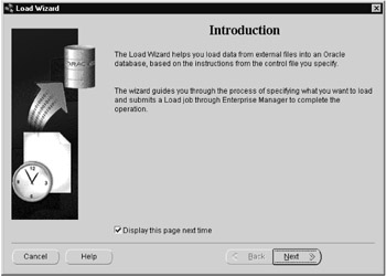
Figure 5.5: The Load Wizard.

You can launch the data management tools by selecting the database tools from the tools menu once the target database is selected in the navigator tree, as shown in Figure 5.6.

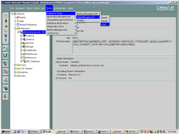
Figure 5.6: Accessing the Load Wizard.

The control file

The control file is a text file that describes the load operation. The role of the control file, which is illustrated in Figure 5.7, is to tell SQL*Loader which data file to load, how to interpret the records and columns, and into what tables to insert the data.

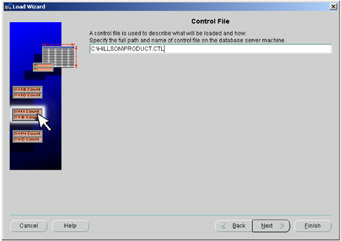
Figure 5.7: The control file.

The control file is written in SQL*Loader's data definition language. The following example shows the control file that would be used to add new product data into the product table in the EASYDW warehouse. The data is stored in the file product.dat. New rows will be appended to the existing table.

 - Load product dimension LOAD DATA INFILE 'product.dat' append INTO TABLE product FIELDS TERMINATED BY ',' OPTIONALLY ENCLOSED BY "'" (product_id,  product_name,  category,  cost_price,  sell_price,  weight,  shipping_charge,  manufacturer,  supplier) 

The data file

The following example shows a small sample of the data file product.dat. Each field is separated by a comma and optionally enclosed in a single quote. Each field in the input file is mapped to the corresponding column in the table. As the data is read, it is converted from the data type in the input file to the data type of the column in the database.

 'SP1242', 'CD LX1','MUSC', 8.90, 15.67, 2.5, 2.95, 'RTG', 'CD Inc' 'SP1243', 'CD LX2','MUSC', 8.90, 15.67, 2.5, 2.95, 'RTG', 'CD Inc' 'SP1244', 'CD LX3','MUSC', 8.90, 15.67, 2.5, 2.95, 'RTG', 'CD Inc' 'SP1245', 'CD LX4','MUSC', 8.90, 15.67, 2.5, 2.95, 'RTG', 'CD Inc' 

The data file is an example of data stored in stream format. A record separator, often a line feed or carriage return/line feed, terminates each record. A delimiter character, often a comma, separates each field. The fields may also be enclosed in single or double quotes.

In addition to the stream format, SQL*Loader supports fixed-length and variable-length format files. In a fixed-length file, each record is the same length. Normally each field in the record is also the same length. In the control file, the input record is described by specifying the starting position, length, and data type. In a variable-length file, each record may be a different length. The first field in each record is used to specify the length of that record.

SQL*Loader modes of operation

Figure 5.8 shows SQL*Loader's two modes of operation: conventional path and direct path.

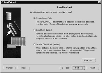
Figure 5.8: SQL*Loader modes of operation.

Conventional path load should only be used to load small amounts of data, such as initially loading a small dimension table, or when loading data with data types not supported by direct path load, such as varrays. The conventional path load issues SQL INSERT statements. As each row is inserted, the indexes are updated, triggers are fired, and constraints are evaluated. When loading large amounts of data in a small batch window, direct path load can be used to optimize performance. Direct path load bypasses the SQL layer. It formats the data blocks directly and writes them to the database files. When running on a system with multiple processors, the load can be executed in parallel, which can result in significant performance gains.

Handling SQL*Loader errors

You can create additional files during the load operation to aid in the diagnosis and correction of any errors that may occur during the load. A log file is created to record the status of the load operation. This should always be reviewed to ensure the load was successful. Copies of the records that could not be loaded into the database because of data integrity violations can be saved in a "bad" file. This file can later be reentered once the data integrity problems have been corrected. If you receive an extract file with more records than you are interested in, you can load a subset of records from the file. The WHEN clause in the control file is used to select the records to load. Any records that are skipped are written to a discard file.

Select which optional files you would like created using the advanced option, as shown in Figure 5.9. In this example, we've selected a bad file and a log file.

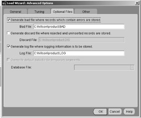
Figure 5.9: SQL*Loader advanced options.

Scheduling the load operation

Enterprise Manager's job scheduling system allows you to create and manage jobs, schedule the jobs to run, and monitor progress. You can run a job once or choose how frequently you would like the job to run. If you will run the job multiple times, you can save the job in Enterprise Manager's jobs library so that it can be rerun in the future. In Figure 5.10, the job will be scheduled to run once, at 11:31 p.m.

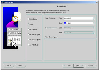
Figure 5.10: Scheduling the load.

Monitoring progress of the load operation

You can monitor the progress of a job while it is running by clicking on jobs in the navigator tree on the Enterprise Manager Console, as shown in Figure 5.11. The Active page lists all jobs that are either running or are scheduled to run. By clicking on the job in the Active Jobs page, information about the job's state and progress can be displayed. Load 0016 has been submitted and will run at 11:31 p.m. The History page contains a list of jobs that have been run previously. You can check to see if the job ran successfully after it has completed and look at the output to see any errors when a job has failed.

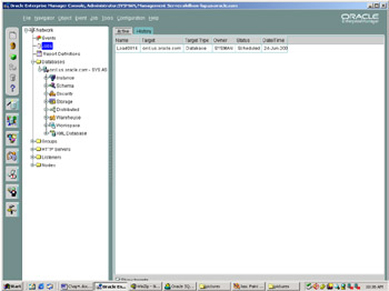
Figure 5.11: Monitoring jobs from the OEM console.

Inspecting the SQL*Loader log

The following example shows a portion of the log file from a sample load session. A total of 159 rows were appended to the product table. Ten records were rejected due to invalid data. Copies of those records can be found in the file product.bad.

 SQL*Loader: Release 9.2.0.1.0 - Production on Mon Jun 24 06:45:47 2002 Copyright (c) 1982, 2002, Oracle Corporation. All rights reserved. Control File:   C:\hillson\product.ctl Data File:      c:\hillson\product.dat Bad File:     C:\hillson\product.BAD Discard File:  none specified  (Allow all discards) Number to load: ALL Number to skip: 0 Errors allowed: 50 Bind array:     64 rows, maximum of 256000 bytes Continuation:    none specified Path used:      Conventional Table EASYDW.PRODUCT, loaded from every logical record. Insert option in effect for this table: APPEND     Column Name  Position   Len  Term  Encl Datatype ---------------- ---------- ----- ---- ---- ---------- PRODUCT_ID            FIRST     *   ,  O(') CHARACTER PRODUCT_NAME           NEXT     *   ,  O(') CHARACTER CATEGORY               NEXT     *   ,  O(') CHARACTER COST_PRICE             NEXT     *   ,  O(') CHARACTER SELL_PRICE             NEXT     *   ,  O(') CHARACTER WEIGHT                 NEXT     *   ,  O(') CHARACTER SHIPPING_CHARGE        NEXT     *   ,  O(') CHARACTER MANUFACTURER           NEXT     *   ,  O(') CHARACTER SUPPLIER               NEXT     *   ,  O(') CHARACTER Record 1: Rejected - Error on table EASYDW.PRODUCT, column PRODUCT_ID. Column not found before end of logical record (use TRAILING NULLCOLS) Record 3: Rejected - Error on table EASYDW.PRODUCT, column PRODUCT_ID. Column not found before end of logical record (use TRAILING NULLCOLS) Record 4: Rejected - Error on table EASYDW.PRODUCT, column WEIGHT. Column not found before end of logical record (use TRAILING NULLCOLS) Record 5: Rejected - Error on table EASYDW.PRODUCT, column SELL_PRICE. Column not found before end of logical record (use TRAILING NULLCOLS) Record 6: Rejected - Error on table EASYDW.PRODUCT, column SHIPPING_CHARGE. Column not found before end of logical record (use TRAILING NULLCOLS) Record 7: Rejected - Error on table EASYDW.PRODUCT, column COST_PRICE. Column not found before end of logical record (use TRAILING NULLCOLS) Record 8: Rejected - Error on table EASYDW.PRODUCT, column SHIPPING_CHARGE. Column not found before end of logical record (use TRAILING NULLCOLS) Record 9: Rejected - Error on table EASYDW.PRODUCT, column COST_PRICE. Column not found before end of logical record (use TRAILING NULLCOLS) Record 106: Rejected - Error on table EASYDW.PRODUCT. ORA-00001: unique constraint (EASYDW.PK_PRODUCT) violated Record 134: Rejected - Error on table EASYDW.PRODUCT. ORA-00001: unique constraint (EASYDW.PK_PRODUCT) violated Table EASYDW.PRODUCT:   159 Rows successfully loaded.   10 Rows not loaded due to data errors.   0 Rows not loaded because all WHEN clauses were failed.   0 Rows not loaded because all fields were null. Space allocated for bind array:  148608 bytes(64 rows) Read   buffer bytes: 1048576 Total logical records skipped:          0 Total logical records read:           169 Total logical records rejected:        10 Total logical records discarded:        0 Run began on Mon Jun 24 06:45:47 2002 Run ended on Mon Jun 24 06:46:14 2002 Elapsed time was:     00:00:27.56 CPU time was:         00:00:00.09 

Optimizing SQL*Loader performance

When loading large amounts of data in a small batch window, a variety of techniques can be used to optimize performance:

• Using direct path load. Formatting the data blocks directly and writing them to the database files eliminates much of the work needed to execute a SQL insert statement. Direct path load requires exclusive access to the table or partition being loaded. In addition, triggers are automatically disabled, and constraint evaluation is deferred until the load completes.

• Disabling integrity constraint evaluation prior to loading the data. When loading data with direct path, SQL*Loader automatically disables all CHECK and REFERENCES integrity constraints. When using parallel direct path load or loading into a single partition, other types of constraints must be disabled. You can manually disable evaluation of not null, unique, and primary-key constraints during the load process, as well. When the load completes, you can have SQL*Loader reenable the constraints, or do it yourself manually.

• Loading the data in sorted order. Presorting data minimizes the amount of temporary storage needed during the load, enabling optimizations to minimize the processing during the merge phase to be applied. To tell SQL*Loader what indexes the data is sorted on, use the SORTED INDEXES statement in the control file.

• Deferring index maintenance. Indexes are maintained automatically whenever data is inserted or deleted or the key column is updated. When loading large amounts of data with direct path load, it may be faster to defer index maintenance until after the data is loaded. You can either drop the indexes prior to the beginning of the load or skip index maintenance by setting SKIP_INDEX_MAINTENANCE= TRUE on the SQL*Loader command line. Index partitions that would have been updated are marked "index unusable," because the index segment is inconsistent with respect to the data it indexes. After the data is loaded, the indexes must be rebuilt.

• Disabling redo logging by using the UNRECOVERABLE option in the control file. By default, all changes made to the database are also written to the redo log so they can be used to recover the database after failures. Media recovery is the process of recovering after the loss of a database file, often due to a hardware failure such as a disk head crash. By disabling redo logging, the load is faster.

  However, if the system fails in the middle of loading the data, you need to restart the load, since you cannot use the redo log for recovery. If you are using Oracle Data Guard to protect your data with a logical or physical standby database, you may not want to disable redo logging. Any data not logged cannot be automatically applied to the standby site.

  After the data is loaded, using the UNRECOVERABLE option, it is important to do a backup to make sure you can recover the data in the future if the need arises.

• Loading the data into a single partition. While you are loading a partition of a partitioned or subpartitioned table, other users can continue to access the other partitions in the table. Loading the April transactions will not prevent users from querying the existing data for January through March. Thus, overall availability of the warehouse is increased.

• Loading the data in parallel. When a table is partitioned, it can be loaded into multiple partitions in parallel. You can also set up multiple, concurrent sessions to perform a load into the same table or into the same partition of a partitioned table.

• Increasing the STREAMSIZE parameter can lead to better direct path load times, since larger amounts of data will be passed in the data stream from the SQL*Loader client to the Oracle server.

• If the data being loaded contains many duplicate dates, using the DATE_CACHE parameter can lead to better performance of direct path load. Use the date cache statistics (entries, hits, and misses) contained in the SQL*Loader log file to tune the size of the cache for future similar loads.

SQL*Loader direct path load of a single partition

Next, we will look at an example of loading data into a single partition. In the EASYDW warehouse, the fact table is partitioned by date. At the end of April, the April sales transactions are loaded into the EASYDW warehouse.

In the following example, we create a tablespace, add a partition to the purchases table, and then use SQL*Loader direct path load to insert the data into the April 2002 partition.

Step 1: Create a tablespace

 SQL> CREATE TABLESPACE purchases_apr2002      DATAFILE 'c:\ora9ir2\oradata\orcl\PURCHASESAPR2002.f' SIZE 5M      REUSE AUTOEXTEND ON      DEFAULT STORAGE      (INITIAL 64K NEXT 64K PCTINCREASE 0 MAXEXTENTS UNLIMITED); 

Step 2: Add a partition

 SQL> ALTER TABLE easydw.purchases      ADD PARTITION purchases_apr2002      VALUES LESS THAN (TO_DATE('30-04-2002', 'DD-MM-YYYY'))      PCTFREE 0 PCTUSED 99      STORAGE (INITIAL 64K NEXT 64K PCTINCREASE 0)      TABLESPACE purchases_apr2002; 

Step 3: Disable all referential integrity constraints and triggers

When using direct path load of a single partition, referential and check constraints on the table partition must be disabled, along with any triggers.

 SQL> ALTER TABLE purchases DISABLE CONSTRAINT fk_time; SQL> ALTER TABLE purchases DISABLE CONSTRAINT fk_product_id; SQL> ALTER TABLE purchases DISABLE CONSTRAINT fk_customer_id; 

The status column in the user_constraints view can be used to determine if the constraint is currently enabled or disabled. Here we can see that the SPECIAL_OFFER constraint is still enabled.

 SQL> SELECT TABLE_NAME, CONSTRAINT_NAME, STATUS      FROM USER_CONSTRAINTS      WHERE TABLE_NAME = 'PURCHASES'; TABLE_NAME  CONSTRAINT_NAME       STATUS ----------- --------------------- -------- PURCHASES   NOT_NULL_PRODUCT_ID   DISABLED PURCHASES   NOT_NULL_TIME         DISABLED PURCHASES   NOT_NULL_CUSTOMER_ID  DISABLED PURCHASES   SPECIAL_OFFER         ENABLED PURCHASES   FK_PRODUCT_ID         DISABLED PURCHASES   FK_TIME               DISABLED PURCHASES   FK_CUSTOMER_ID        DISABLED 7 rows selected.opt 

The status column in the user_triggers view can be used to determine if any triggers must be disabled. There are no triggers on the PURCHASES table.

 SQL> SELECT TRIGGER_NAME, STATUS      FROM ALL_TRIGGERS WHERE TABLE_NAME = 'PURCHASES'; no rows selected 

Step 4: Load the data

The following example shows the SQL*Loader control file to load new data into a single partition. Note that the partition clause is used.

 UNRECOVERABLE LOAD DATA INFILE 'purchases.dat' BADFILE 'purchases.bad' APPEND INTO TABLE purchases PARTITION (purchases_apr2002)  (product_id         position (1-6)        char,  time_key            position (7-17)       date   "DD-MON-YYYY",  customer_id         position (18-25)      char,  purchase_date       position (26-36)      date "DD-MON-YYYY",  purchase_time       position (37-40)      integer external,  purchase_price      position (41-45)      decimal external,  shipping_charge     position (46-49)      integer external,  today_special_offer position (50)         char) 

The unrecoverable keyword is specified, disabling media recovery for the table being loaded. Database changes being made by other users will continue to be logged. After disabling media recovery, it is important to do a backup, to make it possible to recover the data in the future if the need arises. If you attempted media recovery before the backup was taken, you would discover that the data blocks that were loaded have been marked as logically corrupt. To recover the data, you must drop the partition, and reload the data.

Any data that cannot be loaded will be written to the file purchases.bad. Data will be loaded into the purchases_apr2002 partition. This example shows loading a fixed-length file named purchases.dat. Each field in the input record is described by specifying its starting position, its ending position, and its data type. Note that these are SQL*Loader data types, not the data types in an Oracle table. When the data is loaded into the tables, each field is converted to the data type of the column, if necessary.

The following example shows a sample of the purchases data file. The PRODUCT_ID starts in column 1 and is six bytes long. Time_key starts in column 7 and is 17 bytes long. The data mask DD-MON-YYYY is used to describe the input format of the date fields.

 123456789012345678901234567890123456789012345678901       |          |       |          |    |   |   | SP100101-APR-2002AB12345601-APR-2002002428.014.50Y SP100101-APR-2002AB12345701-APR-2002102428.014.50Y 

To invoke SQL*Loader direct path mode from the command line, set direct=true. In this example, skip_index_maintenance is set to true, so the indexes will need to be rebuilt after the load.

 sqlldr USERID=easydw/easydw CONTROL=purchases.ctl LOG=purchases.log DIRECT=TRUE SKIP_INDEX_MAINTENANCE = TRUE 

Step 5: Inspect the log

The following example shows a portion of the SQL*Loader log file from the load operation. Rather than generating redo to allow recovery, invalidation redo was generated to let Oracle know this table cannot be recovered. The indexes were made unusable. The column starting position and length are described.

 SQL*Loader: Release 9.2.0.1.0 - Production on Sun Jun 9 12:43:45 2002 Copyright (c) 1982, 2002, Oracle Corporation. All rights reserved. Control File:   purchases.ctl Data File:      purchases.dat   Bad File:     purchases.bad   Discard File:  none specified  (Allow all discards) Number to load: ALL Number to skip: 0 Errors allowed: 50 Continuation:    none specified Path used:      Direct Load is UNRECOVERABLE; invalidation redo is produced. Table PURCHASES, partition PURCHASES_APR2002, loaded from every logical record. Insert option in effect for this partition: APPEND    Column Name  Position   Len  Term Encl Datatype --------------- ---------- ---- ---- ---- -------- PRODUCT_ID          1:6     6            CHARACTER TIME_KEY            7:17    11           DATE DD-MON-YYYY CUSTOMER_ID        18:25     8           CHARACTER PURCHASE_DATE      26:36    11           DATE DD-MON-YYYY PURCHASE_TIME      37:40     4           CHARACTER PURCHASE_PRICE     41:45     5           CHARACTER SHIPPING_CHARGE    46:49     4           CHARACTER TODAY_SPECIAL_OFFER   50     1           CHARACTER The following index(es) on table PURCHASES were processed: index EASYDW.PURCHASE_PRODUCT_INDEX partition PURCHASES_APR2002 was made unusable due to: SKIP_INDEX_MAINTENANCE option requested index EASYDW.PURCHASE_CUSTOMER_INDEX partition PURCHASES_APR2002 was made unusable due to: SKIP_INDEX_MAINTENANCE option requested index EASYDW.PURCHASE_SPECIAL_INDEX partition PURCHASES_APR2002 was made unusable due to: SKIP_INDEX_MAINTENANCE option requested 

Step 6: Reenable all constraints and triggers and rebuild indexes

After loading the data into a single partition, all references to constraints and triggers must be reenabled. All local indexes for the partition can be maintained by SQL*Loader. Global indexes are not maintained on single partition or subpartition direct path loads and must be rebuilt. In the previous example, the indexes must be rebuilt since index maintenance was skipped. These steps are discussed in more detail later in the chapter.

SQL*Loader parallel direct path load

When a table is partitioned, the direct path loader can be used to load multiple partitions in parallel. Each parallel direct path load process should be loaded into a partition of a table stored on a separate disk, to minimize I/O contention.

Since data is extracted from multiple operational systems, you will often have several input files that need to be loaded into the warehouse. These files can be loaded in parallel and the workload distributed among several concurrent SQL*Loader sessions.

Figure 5.12 shows an example of how parallel direct path load can be used to initially load the historical transactions into the purchases table. You need to invoke multiple SQL*Loader sessions. Each SQL*Loader session takes a different data file as input. In this example, there are three data files, each containing the purchases for one month: January, February, and March. These will be loaded into the purchases table, which is also partitioned by month. Each data file is loaded in parallel into its own partition.

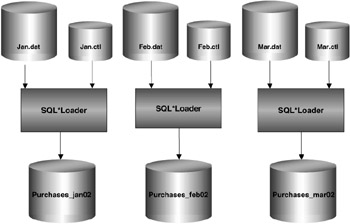
Figure 5.12: SQL*Loader parallel direct path load.

It is suggested that the following steps are followed to load data in parallel using SQL*Loader:

Step 1: Disable all constraints and triggers

Constraints cannot be evaluated, and triggers cannot be fired during a parallel direct path load. If you forget, SQL*Loader will issue an error.

Step 2: Drop all indexes

Indexes cannot be maintained during a parallel direct path load. However, if we are loading only a few partitions out of many, then it is probably better to skip index maintenance and have them marked as unusable instead.

Step 3: Load the data

By invoking multiple SQL*Loader sessions and setting direct and parallel to true, the processes will load concurrently. Depending on your operating system, you may need to put an '&' at the end of each line.

 sqlldr userid=easydw/easydw CONTROL=jan.ctl DIRECT=TRUE PARALLEL=TRUE sqlldr userid=easydw/easydw CONTROL=feb.ctl DIRECT=TRUE PARALLEL=TRUE sqlldr userid=easydw/easydw CONTROL=mar.ctl DIRECT=TRUE PARALLEL=TRUE 

Step 4: Inspect the log

A portion of one of the log files follows. Note that the mode is direct with the parallel option.

 SQL*Loader: Release 9.2.0.1.0 - Production on Sat Jun 15 11:01:21 2002 Copyright (c) 1982, 2002, Oracle Corporation. All rights reserved. Control File:   c:\feb.ctl Data File:      c:\feb.dat   Bad File:     c:\feb.bad   Discard File:  none specified  (Allow all discards) Number to load: ALL Number to skip: 0 Errors allowed: 50 Continuation:    none specified Path used:      Direct - with parallel option. Load is UNRECOVERABLE; invalidation redo is produced. Table PURCHASES, partition PURCHASES_FEB2002, loaded from every logical record. Insert option in effect for this partition: APPEND 

Step 5: Reenable all constraints and triggers

Recreate all indexes. After using parallel direct path load, reenable any constraints and triggers that were disabled for the load. Recreate any indexes that were dropped.

Transformations using SQL*Loader

If you receive extract files that have data in them that you do not want toload into the warehouse, you can use SQL*Loader to filter the rows of interest. You select the records that meet the load criteria by specifying a WHENclause to test an equality or inequality condition in the record. If a record does not satisfy the WHEN condition, it is written to the discard file. The discard file contains records that were filtered out of the load because they did not match any record-selection criteria specified in the control file. Note that these records differ from rejected records written to the BAD file. Discarded records do not necessarily have any bad data. The WHEN clause can be used with either conventional or direct path load.

You can use SQL*Loader to perform simple types of transformations on character data. For example, portions of a string can be inserted using the substring function; two fields can be concatenated together using the CONCAT operator. You can trim leading or trailing characters from a string using the trim operator. The control file in the following example illustrates the use of the WHEN clause to discard any rows where the PRODUCT_ID is blank; it also shows how to uppercase the PRODUCT_ID column.

 LOAD DATA INFILE 'product.dat' append INTO TABLE product WHEN product_id != BLANKS FIELDS TERMINATED BY ',' OPTIONALLY ENCLOSED BY "'" (product_id "upper(:product_id)",  product_name,  category,  cost_price,  sell_price,  weight,  shipping_charge,  manufacturer,  supplier) 

The discard file is specified when invoking SQL*Loader from the command line, as shown, or with the OEM Load Wizard, as seen previously.

 sqlldr userid=easydw/easydw CONTROL=product.ctl LOG=product.log BAD=product.bad DISCARD=product.dis DIRECT=true 

In Oracle 9i these types of transformations can be done with both direct path and conventional path modes. However, since they are applied to each record individually, they do have an impact on the load performance.

SQL*Loader postload operations

After the data is loaded, you may need to process exceptions, reenable constraints, and rebuild indexes.

Inspect the logs

Always look at the logs to ensure the data was loaded successfully. Validate that the correct number of rows have been added.

Process the load exceptions

Look in the .bad file to find out which rows were not loaded. Records that fail NOT NULL constraints are rejected and written to the SQL*Loader bad file.

Reenable data integrity constraints

Ensure referential integrity if you have not already done so. Make sure that each foreign key in the fact table has a corresponding primary key in each dimension table. For the EASYDW warehouse, each row in the PURCHASES table needs to have a valid CUSTOMER_ID in the CUSTOMERS table and a valid PRODUCT_ID in the PRODUCTS table.

When using direct path load, CHECK and REFERENCES integrity constraints were disabled. When using parallel direct path load, all constraints were disabled.

Handle constraint violations

To find the rows with bad data, you can create an exceptions table. Create the table named "exceptions" by running the script UTLEXCPT.SQL. When enabling the constraint, list the table name the exceptions should be written to.

 SQL> ALTER TABLE purchases ENABLE CONSTRAINT fk_product_id                            EXCEPTIONS INTO exceptions; 

In our example, two rows had bad PRODUCT_IDs. A sale was made for a product that does not exist in the product dimension.

 SQL> SELECT * FROM EXCEPTIONS; ROW_ID                  OWNER      TABLE_NAME  CONSTRAINT ------------------------------------------------------------ AAAC/ZAAMAAAAADAAF      EASYDW     PURCHASES   FK_PRODUCT_ID AAAC/ZAAMAAAAADAAI      EASYDW     PURCHASES   FK_PRODUCT_ID 

To find out which rows have violated referential integrity, select the rows from the purchases table where the rowid is in the exception table. In this example, there are two rows where there is no matching product in the products dimension.

 SQL> SELECT * from purchases WHERE row_id in (select row_id from exceptions); PRODUCT_ TIME_KEY CUSTOMER_I PURCHASE_ PURCHASE_TIM PURCHASE_PRICE ------- --------- ---------- --------- ------------ ------------- XY1001  01-MAR-02 AB123457  01-MAR-02   1024        28.01 4.5 Y AB1234  01-MAR-02 AB123456  01-MAR-02     24        28.01 4.5 Y 

Hint: 

It is important to fix any referential integrity constraint problems, particularly if you are using Summary Management, which relies on the correctness of these relationships to perform query rewrite.

Enabling constraints without validation

If integrity checking is maintained in an application or the data has already been cleansed, and you know it will not violate any integrity constraints, enable the constraints with the NOVALIDATE clause. Include the rely clause for query rewrite. Since summary management and other tools depend on the relationships defined by references constraints, you should always define the constraints, even if they are not validated.

 SQL>ALTER TABLE purchases ENABLE NOVALIDATE CONSTRAINT fk_product_id; SQL>ALTER TABLE purchases MODIFY CONSTRAINT fk_product_id RELY; 

Check for unusable indexes

Prior to publishing data in the warehouse, you should check to determine if any indexes are in an unusable state. An index becomes unusable when it no longer contains index entries to all the data. An index may be marked unusable for a variety of reasons, including the following:

• You requested that index maintenance be deferred, using the skip_index_maintenance parameter when invoking SQL*Loader.

• UNIQUE constraints were not disabled when using SQL*Loader direct path. At the end of the load, the constraints are verified when the indexes are rebuilt. If any duplicates are found, the index is not correct and will be left in an "Index Unusable" state.

The index must be dropped and recreated or rebuilt to make it usable again. If one partition is marked UNUSABLE, the other partitions of the index are still valid.

To check for unusable indexes query the table USER_INDEXES as illustrated in the following code. Here we can see that the PRODUCT_PK_INDEX is unusable. If an index is partitioned, its status is N/A.

 SQL> SELECT INDEX_NAME, STATUS FROM USER_INDEXES; INDEX_NAME              STATUS ------------------------------- CUSTOMER_PK_INDEX       VALID I_SNAP$_CUSTOMER_SUM    VALID PRODUCT_PK_INDEX        UNUSABLE PURCHASE_CUSTOMER_INDEX N/A PURCHASE_PRODUCT_INDEX  N/A PURCHASE_SPECIAL_INDEX  N/A PURCHASE_TIME_INDEX     N/A TIME_PK_INDEX           VALID TSO_PK_INDEX            VALID 9 rows selected. 

Next check to see if any index partitions are in an unusable state by checking the table USER_IND_PARTITIONS. In the following example the PURCHASE_PRODUCT_INDEX for the "purchases_apr2002" partition is unusable.

 SQL> SELECT INDEX_NAME, PARTITION_NAME, STATUS FROM      USER_IND_PARTITIONS WHERE STATUS != 'VALID'; INDEX_NAME               PARTITION_NAME      STATUS ------------------------ ------------------- -------- PURCHASE_PRODUCT_INDEX   PURCHASES_JAN2002   USABLE PURCHASE_PRODUCT_INDEX   PURCHASES_FEB2002   USABLE PURCHASE_PRODUCT_INDEX   PURCHASES_MAR2002   USABLE PURCHASE_PRODUCT_INDEX   PURCHASES_APR2002   UNUSABLE 

Rebuild unusable indexes

If you have any indexes that are unusable, you must rebuild them prior to accessing the table or partition. In the following example, the purchases_product_index for the newly added purchases_apr2002 partition is rebuilt.

 SQL> ALTER INDEX purchase_product_index      REBUILD PARTITION purchases_apr2002; 

5.4.2 Loading the warehouse using external tables

An external table is a table stored outside the database in a flat file. The data in an external table can be queried just like a table stored inside the database. You can select columns, rows, and join the data to other tables using SQL. The data in the external table can be accessed in parallel, just like tables stored in the database.

External tables are read-only. No DML operations are allowed, and you cannot create indexes on an external table. If you need to update the data or access it more than once, you can load the data into the database, where you can update it and add indexes to improve query performance. By loading the data into the database, you can manage the data as part of the database. RMAN will not back up the data for any external tables.

Since you can query the data in the external table you have just defined using SQL, you can also load the data using an INSERT SELECT statement. External tables provide an alternative to SQL*Loader to load data from flat files. They can be used to perform more complex transformations while the data is loaded and simplify many of the operational aspects while loading data in parallel and managing triggers, constraints, and indexes. However, in Oracle 9i SQL*Loader direct path load may still be faster in many cases. There are many similarities between the two methods, and if you've used SQL*Loader, you will find it easy to learn to use external tables.

Specifying the location of the data file and log files for an external table

Before creating an external table, a directory object must be created to specify the location of the data files and log files. The data and log files must be on the same machine as the database server, or must be accessible to the server. This is different from SQL*Loader, where the SQL*Loader client sends the data to the server. Directories are created in a single namespace and are not owned by an individual's schema. In the following example, the DBA creates directories for the data and log files.

 SQL> CREATE OR REPLACE DIRECTORY data_file_dir as 'C:\datafiles\'; SQL> CREATE OR REPLACE DIRECTORY log_file_dir as 'C:logfiles\'; 

Read access must be granted to users who will be accessing the data files in the directory. In the following example, the DBA grants read access to user EASYDW.

 SQL> GRANT READ ON DIRECTORY data_file_dir to easydw; SQL> GRANT READ ON DIRECTORY log_file_dir to easydw; 

Looking at the DBA_DIRECTORIES view, we can see the directories that have been defined.

 SQL> SELECT * FROM DBA_DIRECTORIES; OWNER      DIRECTORY_NAME   DIRECTORY_PATH ---------- ---------------- -------------- SYS        LOG_FILE_DIR     c:\logfiles\ SYS        DATA_FILE_DIR    c:\datafiles\ 

Creating an external table

In order to create an external table you must specify the following:

• The metadata, which describes how the data looks to Oracle, including the external table name, the column names, and Oracle data types. These are the names you will use in the SQL statements to access the external table. Metadata is stored in the Oracle data dictionary. In the example shown in Figure 5.13, the external table name is NEW_PRODUCTS. The data is stored outside the database. This differs from the other regular tables in the database, where the data and metadata are both stored in the database.

  
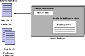
  Figure 5.13: External table.

• The access parameters, which describe how the data is stored in the external file, where it is located, its format, and how to identify the fields and records. The information is similar to what is stored in a SQL*Loader control file. The access driver uses the access parameters. An example of the access parameters is shown in the CREATE EXTERNAL TABLE statement.

In Oracle 9i there is only one type of access driver, called ORACLE_LOADER, which provides read-only access to flat files. It is specified in the TYPE clause on the CREATE EXTERNAL TABLE statement.

The following example shows the SQL to create an external table. The CREATE TABLE ORGANIZATION EXTERNAL clause is used. The metadata describing the column names and data types are listed. The TYPE clause lists the type of access driver and begins the description of how the file is stored on disk. Each field is separated by a comma and optionally enclosed in an apostrophe. The location of the data file, log file, and bad files is specified. By specifying the parallel clause, the data will be loaded in parallel.

 CREATE TABLE new_products (product_id             VARCHAR2(8),  product_name           VARCHAR2(30),  category               VARCHAR2(4),  cost_price             NUMBER (6,2),  sell_price             NUMBER (6,2),  weight                 NUMBER (4,2),  shipping_charge        NUMBER (5,2),  manufacturer           VARCHAR2(20),  supplier               VARCHAR2(10)) ORGANIZATION EXTERNAL (TYPE ORACLE_LOADER    DEFAULT DIRECTORY data_file_dir    ACCESS PARAMETERS (RECORDS DELIMITED BY NEWLINE                     CHARACTERSET US7ASCII                     BADFILE log_file_dir:'product.bad'                     LOGFILE log_file_dir:'product.log'                     FIELDS TERMINATED BY ','                     OPTIONALLY ENCLOSED BY "'")                     LOCATION ('product.dat'))                     REJECT LIMIT UNLIMITED PARALLEL; 

A portion of the data file, product.dat is shown in the following example. Each field is separated by a comma and optionally enclosed in a single quote. As the data is read, each field in the input file is mapped to the corresponding columns in the external table definition. As the data is read, it is converted from the data type of the input file to the data type of the column in the database as necessary.

 'SP1000','Camera','ELEC',45.67,67.23,15.00,4.50,'Ricoh','Ricoh' 'SP1001','APS Camera','ELEC',24.67,36.23,5.00,4.50,'Ricoh','Ricoh' 'SP1010','Camera','ELEC',35.67,47.89,5.00,4.50,'Agfa','Agfa' 

After executing the CREATE TABLE command shown previously, the metadata for the NEW_PRODUCTS table is stored in the database. The table is as follows.

 SQL> DESCRIBE new_products;  Name                  Null?    Type  --------------------- -------- ------------  PRODUCT_ID                     VARCHAR2(8)  PRODUCT_NAME                   VARCHAR2(30)  CATEGORY                       VARCHAR2(4)  COST_PRICE                     NUMBER(6,2)  SELL_PRICE                     NUMBER(6,2)  WEIGHT                         NUMBER(4,2)  SHIPPING_CHARGE                NUMBER(5,2)  MANUFACTURER                   VARCHAR2(20)  SUPPLIER                       VARCHAR2(10) 

The USER_EXTERNAL_TABLES dictionary view shows what external tables have been created, along with a description of them. The USER_EXTERNAL_LOCATIONS dictionary view shows the location of the data file.

 SQL> SELECT TABLE_NAME, TYPE_NAME, DEFAULT_DIRECTORY_NAME      FROM USER_EXTERNAL_TABLES; T0ABLE_NAME   TYPE_NAME       DEFAULT_DIRECTORY_NAME ------------- --------------- ---------------------- NEW_PRODUCTS  ORACLE_LOADER    DATA_FILE_DIR SQL> SELECT * FROM USER_EXTERNAL_LOCATIONS; TABLE_NAME    LOCATION     DIR DIRECTORY_NAME ------------- ------------ --- -------------- NEW_PRODUCTS  product.dat  SYS DATA_FILE_DIR 

Accessing data stored in an external table

After defining the external table, it can be accessed using SQL just as if it were any other table in the database, although the data is being read from the file outside the database. A portion of the output is as follows:

 SQL> SELECT * FROM NEW_PRODUCTS; PRODUCT PRODUCT       CAT COST  SELL WEIGHT SHIPPING MANUF SUPPL ID      NAME              PRICE PRICE       CHARGE ------------------------------------------------------------------ SP1000 Camera         ELEC 45.67 67.23 15     4.5    Ricoh Ricoh SP1001 APS  Camera    ELEC 24.67 36.23  5     4.5    Ricoh Ricoh SP1010 Camera         ELEC 35.67 47.89  5     4.5    Agfa Agfa 

Loading data from an external table

The next example will use the INSERT/SELECT statement to load the data into the PRODUCT dimension table. It is very easy to perform transformations during the load using SQL functions and arithmetic operators. In this example, after the data file was created, the cost of fuel rose, and our shipping company increased the shipping rates by 10 percent. In this example, data is loaded into the EASYDW.PRODUCT table by selecting the columns from the NEW_PRODUCTS external table. The shipping charge is increased by 10 percent for each item as the data is loaded.

 SQL> INSERT INTO easydw.product            (product_id, product_name, category, cost_price,             sell_price, weight, shipping_charge, manufacturer,             supplier)      SELECT product_id, product_name, category, cost_price,             sell_price, weight,             (shipping_charge + (shipping_charge * .10)),             manufacturer, supplier FROM new_products; 

The data has now been loaded into the EASYDW.PRODUCT table, and we can see that the shipping charge increased from $4.50 to $4.95 for the items displayed.

 SQL> select * from easydw.product; PRODUCT PRODUCT       CAT COST  SELL WEIGHT SHIPPING MANUF SUPPL ID      NAME              PRICE PRICE       CHARGE ------------------------------------------------------------------ SP1000 Camera         ELEC 45.67 67.23 15     4.95   Ricoh Ricoh SP1001 APS Camera     ELEC 24.67 36.23  5     4.95   Ricoh Ricoh SP1010 Camera         ELEC 35.67 47.89  5     4.95   Agfa Agfa 

Loading data in parallel using external tables

Another advantage of using external tables is the ability to load the data in parallel without having to split a large file into smaller files and start multiple sessions, as you must do with SQL*Loader. The degree of parallelism is set using the standard parallel hints or with the PARALLEL clause when creating the external table, as shown previously. The output of an EXPLAIN PLAN shows the parallel access.

 SQL> EXPLAIN PLAN FOR INSERT INTO easydw.product            (product_id, product_name, category, cost_price,             sell_price, weight, shipping_charge, manufacturer,             supplier)      SELECT product_id, product_name, category, cost_price,             sell_price, weight,             (shipping_charge + (shipping_charge * .10)),             manufacturer, supplier FROM new_products; 

The utlxplp.sql procedure is used to show the EXPLAIN PLAN output with the columns pertaining to parallel execution, which have been edited and and are shown in bold type for readability.

 SQL> @c:\ora9iR2\rdbms\admin\utlxplp.sql PLAN_TABLE_OUTPUT ---------------------------------------------------------------- |Id|Operation|Name    |Rows|Bytes|Cost |TQ   |IN-OUT|PQ Distrib| ---------------------------------------------------------------- | 0|INSERT   |        |8168| 781K|   4 |     |      |          | | 1|EXTERNAL |NEW_    |8168| 781K|   4 |20,00|P->S  |QC        | |  |TABLE    |PRODUCTS|    |     |     |     |      |RANDOM    | |  |ACCESS   |        |    |     |     |     |      |          | |  |FULL     |        |    |     |     |     |      |          | ---------------------------------------------------------------- 

Loading the dimensions using SQL MERGE

When loading new data into existing dimension tables, you may need to add new rows and make changes to existing rows. In the past, special programming logic was required to differentiate a new row from a changed row. A new capability was added in Oracle 9i, which makes this process much easier: the SQL MERGE. This is often called an "upsert." If a row exists, update it. If it doesn't exist, insert it.

In the following example, new data is added to the customer dimension. The input file has both new customers who have been added, as well as changes to existing customer data. In this case, there is no need to retain the old customer information, so it will be updated. An external table, named CUSTOMER_CHANGES, is created for the file containing the updates to the customer dimension.

 CREATE TABLE easydw.customer_changes (customer_id            VARCHAR2(10),  town                   VARCHAR2(10),  county                 VARCHAR2(10),  postal_code            VARCHAR2(10),  dob                    DATE,  country                VARCHAR2(20),  occupation             VARCHAR2(10)) ORGANIZATION EXTERNAL (TYPE oracle_loader       DEFAULT DIRECTORY data_file_dir       ACCESS PARAMETERS (RECORDS DELIMITED BY NEWLINE                          CHARACTERSET US7ASCII                          BADFILE log_file_dir:'cus_changes.bad'                          LOGFILE log_file_dir:'cust_changes.log'                          FIELDS TERMINATED BY ','                          OPTIONALLY ENCLOSED BY "'")                          LOCATION ('customer_changes.dat'))                          REJECT LIMIT UNLIMITED NOPARALLEL; 

Instead of using an insert statement to load the data, the MERGE statement is used. The MERGE statement has two parts. When the customer_id in the customer_table matches the customer_id in the customer_changes table, the row is updated. When the customer_id's do not match, a new row is inserted.

 MERGE INTO easydw.customer c USING easydw.customer_changes cc ON (c.customer_id = cc.customer_id) WHEN MATCHED THEN UPDATE SET c.town=cc.town, c.county=cc.county, c.postal_code=cc.postal_code,       c.dob=cc.dob, c.country=cc.country, c.occupation=cc.occupation WHEN NOT MATCHED THEN INSERT      (customer_id, town, county, postal_code,       dob, country, occupation)      VALUES      (cc.customer_id, cc.town, cc.county, cc.postal_code,       cc.dob, cc.country, cc.occupation); 

Before merging the customer changes, we had 45 customers.

 SQL> SELECT COUNT(*) FROM customer;   COUNT(*) ----------         45 

Once the external table is created, we can use SQL to look at the customer_changes data file. The first two are rows that will be updated. The first customer was previously a housewife and is now returning to work as an engineer. The second customer moved from Soton2 to Soton. The last two rows are new customers who will be inserted.

 SQL> SELECT * FROM customer_changes; CUSTOMER_ID TOWN   COUNTY  POSTAL_CODE DOB    COUNTRY  OCCUPATION ----------- ------ ------- ----------- ------ -------- ---------- AB123459   Soton   Hants   SO11TF     23-SEP-27 UK      ENGINEER AB123460   Soton   Hants   SO11TF     23-SEP-27 UK      HOUSEWIFE AA114778   London  London  W11QC      14-APR-56 UK      ENGINEER AA123478   London  London  W11QC      14-APR-56 UK      ENGINEER 

Looking at a portion of the customer dimension, we can see the rows where the CUSTOMER_ID column matches the CUSTOMER_ID column in the CUSTOMER_CHANGES external table. These rows will be updated.

 SQL> SELECT * FROM customer; CUSTOMER_ID TOWN   COUNTY  POSTAL_CODE DOB    COUNTRY  OCCUPATION ----------- ------ ------- ----------- ------ -------- ---------- AB123459   Soton   Hants   SO11TF     23-SEP-27 UK      HOUSEWIFE AB123460   Soton2  Hants   SO11TF     23-SEP-27 UK      HOUSEWIFE 

After the MERGE, we now have 47 customers. A portion of the output, just the rows that have changed, are displayed from the customer table.

 SQL> SELECT COUNT(*) FROM customer;   COUNT(*)   --------        47 SQL> SELECT * FROM customer; CUSTOMER_ID TOWN   COUNTY  POSTAL_CODE DOB    COUNTRY  OCCUPATION ----------- ------ ------- ----------- ------ -------- ---------- AB123459   Soton   Hants   SO11TF     23-SEP-27 UK      ENGINEER AB123460   Soton   Hants   SO11TF     23-SEP-27 UK      HOUSEWIFE AA114778   London  London  W11QC      14-APR-56 UK      ENGINEER AA123478   London  London  W11QC      14-APR-56 UK      ENGINEER 

In this example the MERGE statement was used with external tables. It can also be used with any user tables.

5.4.3 Loading the warehouse using transportable tablespaces

The fastest way to move data from one Oracle database to another is by using transportable tablespaces. Transportable tablespaces provide a mechanism to move one or more tablespaces from one Oracle database into another. Rather than processing the data a row at time, the entire file or set of files is physically copied from one database and integrated into the second database by importing the metadata describing the tables in the files. In addition to data in tables, the indexes can also be moved.

Because the data is not unloaded and reloaded, it can be moved quickly, but it cannot be converted to another format. Thus, in Oracle 9i, you can transport tablespaces between Oracle databases that use the same character set and the same operating system. If any types of data conversions are necessary, another mechanism must be used.

Transportable tablespaces can be used to move data from the operational database to the staging area if you are using an Oracle database to do your staging. Transportable tablespaces are also useful to move data from the data warehouse to a dependent data mart.

Figure 5.14 shows the steps involved in using transportable tablespaces. These steps are as follows:

1. Create a new tablespace.

2. Move the data you want to transfer into its own tablespace.

3. Alter the tablespace to read only.

4. Use the export utility to unload the metadata describing the objects in the tablespace.

5. Copy the data files and export dump file containing the metadata to the target system.

6. Use the import utility to load the metadata descriptions into the target database.

7. Alter the tablespace to read write.

8. Perform transformations.

9. Move the data from the staging area to the warehouse fact table.

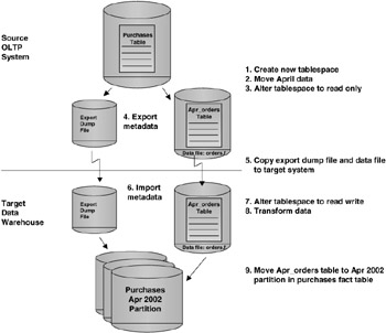
Figure 5.14: Transportable tablespaces.

This section will talk about steps 1–7. In the next sections, we'll look at steps 8 and 9.

One of the sources for data in the EASYDW warehouse is an Oracle 9i order-processing system. In this example, the order-entry system has a record for every order stored in the purchases table. At the end of April, all the orders for April 2002 will be copied into a new table called APR_ORDERS in the ORDERS tablespace stored in the datafile "orders.f."

Here are the steps that are required to transport a tablespace from one database to another.

Step 1: Create a tablespace in the OLTP system

Choose a name that is unique on both the source and target system. In this example, the tablespace ORDERS is created, and its corresponding data file is "orders.f."

 CREATE TABLESPACE orders datafile 'c:\ora9ir2\oradata\orcl\orders.f' SIZE 5M REUSE AUTOEXTEND ON DEFAULT STORAGE (INITIAL 64K PCTINCREASE 0 MAXEXTENTS UNLIMITED); 

Step 2: Move the data for April 2002 into a table in the newly created tablespace

In this example, a table is created and populated using the CREATE TABLE AS SELECT statement. It is created in the ORDERS tablespace. In this example, there are 15,004 orders for April.

 SQL> CREATE TABLE apr_orders TABLESPACE orders AS      SELECT * FROM purchases WHERE      purchase_date BETWEEN '01-APR-2002' AND '30-APR-2002'; SQL> SELECT COUNT(*) FROM apr_orders;   COUNT(*)   --------     15004 

Each tablespace must be self-contained and cannot reference anything outside the tablespace. If there was a global index on the April ORDERS table, it would not be self-contained, and the index would have to be dropped before the tablespace could be moved.

Step 3: Alter the tablespace so that it is read only

If you do not do this, the export in the next step will fail.

 ALTER TABLESPACE orders READ ONLY; 

Step 4: Export the metadata

Using the EXPORT command, the metadata definitions for the orders tablespace are extracted and stored in the export dump file "expdat.dmp."

 exp 'system/manager as sysdba' TRANSPORT_TABLESPACE=y       TABLESPACES=orders TRIGGERS=n CONSTRAINTS=n GRANTS=n       FILE=expdat.dmp LOG=export.log 

When transporting a set of tablespaces, you can choose to include referential integrity constraints. However, if you do include these, you must move the tables with both the primary and foreign keys.

Hint: 

When exporting and importing tablespaces, be sure to connect" as sysdba."

The following example is a copy of the log file, export.log, generated from the export. Only the tablespace metadata is exported, not the data.

 Connected to: Oracle9i Enterprise Edition Release 9.2.0.1.0 - Production With the Partitioning, OLAP and Oracle Data Mining options JServer Release 9.2.0.1.0 - Production Export done in WE8MSWIN1252 character set and AL16UTF16 NCHAR character set Note: table data (rows) will not be exported Note: grants on tables/views/sequences/roles will not be exported Note: constraints on tables will not be exported About to export transportable tablespace metadata... For tablespace ORDERS ... . exporting cluster definitions . exporting table definitions . . exporting table                     APR_ORDERS . end transportable tablespace metadata export Export terminated successfully without warnings. 

Step 5: Transport the tablespace

Now copy the data file, orders.f, and the export dump file, expdat.dmp, to the physical location on the system containing the staging database. You can use any facility for copying flat files, such as an operating system copy utility or FTP. These should be copied in binary mode, since they are not ASCII files.

In our example, orders.f was copied to c:\ora9ir2\oradata\orcl\orders.f on the staging system using FTP.

Step 6: Import the metadata

By importing the metadata, you are plugging the tablespace into the target database.

 imp 'system/manager AS SYSDBA' TRANSPORT_TABLESPACE=Y Datafiles='c:\ora9ir2\oradata\orcl\orders.f' FILE=expdat.dmp LOG=import.log 

Check the import log to ensure no errors have occurred. Note that the transportable tablespace metadata was imported.

 Connected to: Oracle9i Enterprise Edition Release 9.2.0.1.0 - Production With the Partitioning, OLAP and Oracle Data Mining options JServer Release 9.2.0.1.0 - Production Export file created by EXPORT:V09.02.00 via conventional path About to import transportable tablespace(s) metadata... import done in WE8MSWIN1252 character set and AL16UTF16 NCHAR character set . importing SYS's objects into SYS . importing SYSTEM's objects into SYSTEM . . importing table                   "APR_ORDERS" Import terminated successfully without warnings. 

Check the count to ensure that the totals match the OLTP system.

 SQL> SELECT COUNT(*) FROM apr_orders;   COUNT(*) ----------      15004 

Step 7: Alter the ORDERS tablespace so that it is in read/write mode

You are ready to perform your transformations!

 SQL> ALTER TABLESPACE orders READ WRITE; 

As you can see by following these steps, the individual rows of a table are never unloaded and reloaded into the database. Thus, using transportable tablespaces is the fastest way to move data between two Oracle databases.