8.2 What-if analysis using data tables | Microsoft Office Automation with Visual FoxPro

What-if analysis using data tables

The easiest form of what-if analysis is to add some data cells to your spreadsheet along with a formula that uses those data cells, and then change the value of the data cells to see how the formula changes. This simple analysis feature keeps many Excel users happy.

The drawback to this approach is that you see only one result at a time. Sometimes it would be nice to see the results of a series of values for one of the data cells all at the same time. For example, it s easier to figure out how much to sell an item for if you can see the retail prices for a variety of markup values. You might be looking at a widget that has a cost of $5.96. You d like to see the sale price for this item with markups of 15, 20, 25, 30, and 35 percent. Using a data table, you can develop a chart like the one shown in Figure 5. A data table is built from a range containing a formula and the values to plug into the formula in a column (or row).

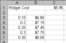
Figure 5. A simple data table. Data tables show multiple values of one (or two) of the cells used in a formula. In this case, the formula, =C1 * (1 + A3), is stored in cell B3. Successive lines in the table replace cell A3 in the formula with the value in column A.

Let s look at how this table is set up. First, we have the Widget Cost in cell C1. The markup values to analyze are in A3:A7. The formula to use is "=C1 * (1 + A3)", and it s in cell B3. Here s the code to get the data set up. If you re following along in FoxPro with the book, be sure to close the last spreadsheet and start a new sheet with the first three lines of the code:

RELEASE oPivotTable, oBook, oSourceData, oDestination

oBook = oExcel.Workbooks.Add

oSheet = oBook.Sheets[1]

* Set up and format the Widget Cost row

oSheet.Range("A1") = "Widget Cost"

oSheet.Range("C1") = 5.96

oSheet.Range("C1").NumberFormat = "$#,###.#0"

* Add the markup values to analyze

oSheet.Range("A3") = ".15"

oSheet.Range("A4") = ".20"

oSheet.Range("A5") = ".25"

oSheet.Range("A6") = ".30"

oSheet.Range("A7") = ".35"

* Put in the formula, and format the cells (including the data table

* results) to look like currency.

oSheet.Range("B3") = "=C1 * (1 + A3)"

oSheet.Range("B3:B7").NumberFormat = "$#,###.#0"

One way to fill in the rest of the values is to slightly modify this formula to "=$C$1 * (1 + A3)" and copy it down the rest of the cells. Better yet, we could use one line to set up a data table. Use the Table method of the Range object. The layout of the data has been carefully set up to ensure that the data table will work. The formula is one column to the right of and one row up from the topmost value in the column of values to substitute into the formula. The value that we re substituting, in A3, can be anywhere in the workbook. However, because it s one of the values under consideration, it makes sense to make it look like the first value in the table this spot in the table could be blank if the value was somewhere else.

The Table method works on a range, which is the rectangular area including the formula and the values; there should be at least two rows and two columns. In the case of this example, the range is A3:B7. The method takes two parameters. Each is a range found in the formula the first is the range to replace with the values found in the rows in the data table range, and the second is the range to replace with the values found in the columns of the data table. In this example, only columns are used. The following line produces the data table shown in Figure 5:

oSheet.Range("A3:B7").Table("",oSheet.Range("A3"))

So why set up a data table when you can copy the formula almost as easily? There are quite a number of reasons. Perhaps the nicest reason is that you can change the formula in the data table (cell B3, in our example), and the rest of the table will change. If you examine the contents of cells B4:B7, you see that they contain the value {=TABLE(,A3)}. This means that the value of each cell is calculated from the formula at the top of the table (or the leftmost value, if using rows). No need to copy the formula to the rest of the cells if you want to change the formula.

Another reason that data tables are useful is that you can include more formulae in successive columns of the table. For example, say you d also like to compare the Wadget costs at the same markups. Add the Wadget data to the first row, and add the Wadget formula to C3, which is next to the Widget formula in B3:

* Set up and format the Wadget Cost row

oSheet.Range("E1") = "Wadget Cost"

oSheet.Range("G1") = 4.23

oSheet.Range("G1").NumberFormat = "$#,###.#0"

* Put in the formula, and format the cells (including the data table

* results) to look like currency.

oSheet.Range("C3") = "=G1 * (1 + A3)"

oSheet.Range("C3:C7").NumberFormat = "$#,###.#0"

Now you re ready to add the data table. Expand the range to include the columns for the values, the Widget formula, and the Wadget formula.

oSheet.Range("A3:C7").Table("",oSheet.Range("A3"))

Figure 6 shows the results. No extra effort is expended to copy formulae, and you can still change either (or both) formulae and affect the respective columns in the table.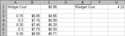

Figure 6. A data table with two calculated columns. Column B shows the Widgets and column C shows the Wadgets, with costs calculated from column A. You can have many formulae in row 3 to include in the data table just include the columns in the Range object.

Yet another way to construct a data table is to allow changes in two cells in the formula. In this case, the values for the first cell go in the first column of the table, and the values for the second cell go in the first row of the table (starting in column 2). The cell at the first row and column contains the formula. Listing 2 (XLData2.PRG in the Developer Download files available at www.hentzenwerke.com) shows the code to set up the data table shown in Figure 7. This data table depicts the cost to purchase up to four Widgets and includes the shipping cost (which is a flat cost, regardless of the number of Widgets purchased). The Quantity variable is placed in a column, and the Shipping Costs variable is placed in a row.

Listing 2. Setting up a data table with two variables.
* Clean out any existing references to servers.

* This prevents memory loss to leftover instances.

RELEASE ALL LIKE o*

* For demonstration purposes, make oExcel and oBook

* and oSheet available after this program executes.

PUBLIC oExcel, oBook, oSheet

#DEFINE xlEdgeBottom 9

#DEFINE xlEdgeRight 10

#DEFINE xlContinuous 1

oExcel = CREATEOBJECT("Excel.Application")

oExcel.Visible = .T.

oBook = oExcel.Workbooks.Add()

oSheet = oBook.Sheets[1]

* Set up the variables for the formula

oSheet.Range("A1").Value = "Widget Cost"

oSheet.Range("C1").Value = 7.00

oSheet.Range("C1").NumberFormat = "$###.00"

oSheet.Range("C1").Name = "Cost"

oSheet.Range("A2").Value = "Widget Quantity"

oSheet.Range("C2").Value = 1

oSheet.Range("C2").Name = "Quantity"

oSheet.Range("A3").Value = "Shipping"

oSheet.Range("C3").Value = 2.00

oSheet.Range("C3").NumberFormat = "$###.00"

oSheet.Range("C3").Name = "Shipping"

* Set up the row headings

oSheet.Range("C5").Value = "Shipping Costs"

oSheet.Range("C6").Value = "Ground"

oSheet.Range("D6").Value = "Overnight"

oSheet.Range("E6").Value = "2-Day"

* Set up the row values

oSheet.Range("C7").Value = 2

oSheet.Range("D7").Value = 16

oSheet.Range("E7").Value = 8

* Set up the column headings

oSheet.Range("A8").Value = "Widget"

oSheet.Range("A9").Value = "Quantity"

* Set up the column values

oSheet.Range("B8").Value = 1

oSheet.Range("B9").Value = 2

oSheet.Range("B10").Value = 3

oSheet.Range("B11").Value = 4

* Add the formula

oSheet.Range("B7").Value = "=(Cost * Quantity) + Shipping"

* Create the table

oSheet.Range("B7:E11").Table(oSheet.Range("Shipping"), oSheet.Range("Cost"))

* Format the cells for currency

oSheet.Range("C7:E11").NumberFormat = "$###.00"

* Put in the cell borders for clarity

oSheet.Range("A7:E7").Borders(xlEdgeBottom).LineStyle = xlContinuous

oSheet.Range("B5:B11").Borders(xlEdgeRight).LineStyle = xlContinuous

Try changing the values in the formula cells the widget cost (C1), the shipping costs (C7:E7), and the widget quantity (B8:B11). You can also change the formula in B7. Instead of a flat shipping cost, you could change it to a per-item shipping cost by changing the formula to "=(Cost * Quantity) + (Quantity * Shipping)." Watch how the appropriate parts of the table change without having to copy formulae. It s pretty cool.

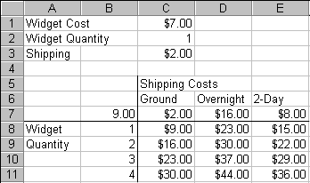
Figure 7. A two-variable data table. The formula is "=(Cost * Quantity) + Shipping" (without range names, it s "=(C1*C2) + C3)"), and it s contained in cell B7. The table range is B7:E11. The values in the column substitute for C2 in the formula, while the values in the row substitute for C3. If you change the widget cost (C1), the shipping costs (C7:E7), or the quantities (B8:B11), the entire table is recalculated to reflect the values.