Hack 52 Create Charts That Adjust to Data

   

Hack 52 Create Charts That Adjust to Data

Your charts can include and plot new data automatically, the moment you add the data to your spreadsheet .

If you use dynamic named ranges in lieu of range references, your chart will plot any new data the moment you add it to your worksheet. To see how this works, begin with a clean worksheet and set up some data similar to that shown in Figure 5-7.

Figure 5-7. Data to be charted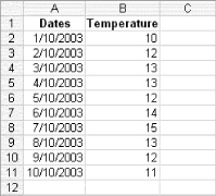

To create the chart and make it dynamic, you need to add two named ranges. One of the named ranges is for the category labels (Dates) and the other is for the actual data points (Temperature).

If you are unsure as to how to insert a dynamic named range, check out [Hack #42], which discusses this in full.

Create a dynamic named range called TEMP_DATES for the dates in column A by selecting Insert Name Define, and type this formula:

 =OFFSET($A,1,0,COUNTA($A:$A)-1,1) 

Notice that you included a -1 immediately after the COUNTA argument. This ensures that the heading is not included in the named range for that particular series.

In this example, you referenced the entire column A as the COUNTA argument ($A:$A). In older versions of Excel, it is often good practice to restrict this range to a much smaller group of cells, so as not to add unnecessary overhead to calculations. In other words, you could be forcing Excel to look in potentially thousands of cells unnecessarily. Some of Excel's functions are smart enough to know which cells are dirty (contain data), but some functions are not. However, this is slightly less necessary with more recent versions of Excel, as Excel has improved its handling of large ranges.

Next, for the Temperature readings in column B, set up another dynamic range called TEMP_READINGS , using this formula:

 =OFFSET($B,0,0,COUNTA($B:$B)-1,1) 

Now you can create the chart using the dynamic named ranges you created in lieu of cell references.

Highlight the data (range $A$1:$B$11), then select the Chart icon on the Standard toolbar. From Step 1 of the Wizard, select the chart type you want to use (for this example we will use a column), and click Next. In Step 2 of the Wizard, you will be presented with two tabs: Data Range and Series. Series is the one you want. Delete the formula that presently sits in the Value: box, and enter the following:

 =Sheet1!TEMP_READINGS 

It is very important to include the Sheet name of your workbook in your formula references. If you don't, you will not be able to enter the named range in your formula.

Finally, delete the formula that presently sits under Category X Labels: and enter the following:

 =Sheet1!TEMP_DATES 

Complete the rest of the Chart Wizard to finish your chart, making any changes required along the way. The result will look like Figure 5-8.

Figure 5-8. Dynamic named ranges in lieu of static range references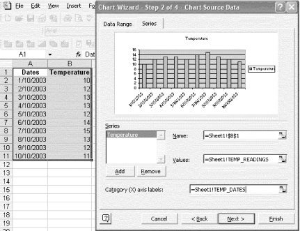

Once this chart is set up, every time you include another entry in either column A (Dates) or column B (Temperature), it will be added to your chart automatically.

Plotting the Last x Number of Readings

Another type of named range that you can use with charts is one that picks up only the last 10 readings (or whatever number you nominate ) in a series of data. Try this using the same data you used in the first part of this hack.

For the dates in column A, set up a dynamic named range called TEMP_DATES_10DAYS that references the following:

 =OFFSET($A,COUNTA($A:$A)-10,0,10,1) 

For readings in column B, set up another dynamic named range called TEMP_READINGS_10DAYS and enter the following:

 =OFFSET(Sheet1!$A,COUNTA(Sheet15!$A:$A)-10,1,10,1) 

If you want to vary the number of readingsto 20, for instancechange the last part of the formula so that it reads as follows :

 =OFFSET(Sheet1!$A,COUNTA(Sheet15!$A:$A)-20,1,20,1) 

Using dynamic named ranges with your charts gives you enormous flexibility and will save you loads of time tweaking your charts whenever you make an additional entry to your source data.

Andy Pope