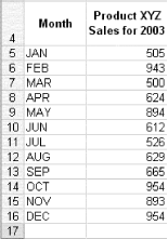
Hack 53 Interact with Your Charts Using Custom Controls

To make your chart truly interactive, you can use one or more dynamic ranges in your chart and then use either a scrollbar or a drop-down list from the Forms toolbar to reveal the figures your readers want to peruse .

As you saw in the previous hack, you can use dynamic named ranges to add flexibility to your charts. But you also can use dynamic named ranges to create interfaces controlling which data the chart plots. By linking dynamic named ranges to custom controls, you enable users to change the chart data by using the control, which simultaneously will update the data in the worksheet or vice versa.

Using a Dynamic Named Range Linked to a Scrollbar

In this example, you will use a scrollbar to reveal monthly figures over a 12-month period. The scrollbar is used to alter the number of months reported . The scrollbar's value also is used in a dynamic range, which in turn is used as the data source of the chart.

To begin, set up some data similar to that shown in Figure 5-9.

Figure 5-9. Worksheet data for dynamic chart linked to scrollbar

Create a dynamic named range by selecting Insert Name Define and call it SALES_PERIOD . In the Refers To: box, type the following:

 =OFFSET($B,0,0,$C,1)

By using the OFFSET function, you can use cell $C$5 to force the referenced range for SALES_PERIOD to expand both up and down as the number in $C$5 changes. In other words, changing the number in $C$5 to the number 5 would force the range to incorporate B5:B10.

If you do not want the user to see cell C5, you can take this a step further and hide the contents of $C$5 by right-clicking it and selecting Format Cells Custom. Enter the format ;;; , and then click OK. In Figure 5-9, the contents of cell C5 are hidden.

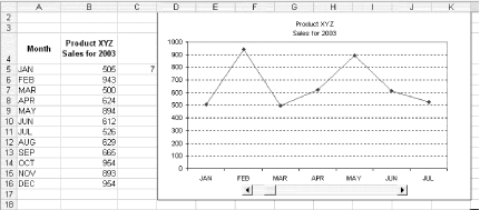
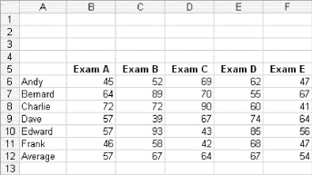
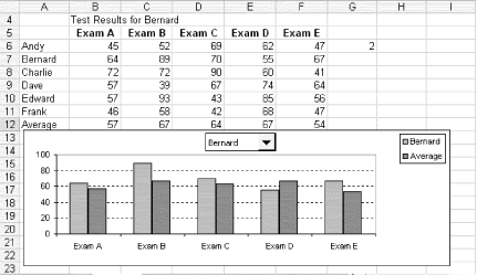
Create a chart (a line chart or a column chart works best). When you get to Step 2 of the Chart Wizard, select the Series tab and change the Formula Reference in the Values: box so that it reads =<Workbook.xls>!SALES_PERIOD . Doing this will make your chart dynamic.

Once you have created your chart, you will need to insert a scrollbar from the Forms toolbar. The easiest way to do this is to right-click the gray area at the top of the screen (this is known as the Toolbar area) and select Forms. This will bring the Forms toolbar onto the screen.

Click the scrollbar icon to select it. Once you have inserted a scrollbar, select it and move it onto your chart. Now right-click it and select Format Control, change the minimum value to 1 , change the maximum value to 12 , and set the cell link to $C$5 . The resulting chart will look like that shown in Figure 5-10.

Figure 5-10. Dynamic chart linked to scrollbar

Using a Dynamic Named Range Linked to a Drop-Down List

Another variation is to link to a drop-down list. Starting with some data such as that shown in Figure 5-9, you will add a dynamic range that will be used as a data source for the chart. The dynamic range will be linked to a drop-down list you can use to view one student's test results from those of a group of students. You will use the drop-down list to select the name of the student whose results you want to view.

Use the formula =AVERAGE(B6:B11) in cell B12 and copy it across to cell F12, as shown in Figure 5-11.

Figure 5-11. Dynamic chart linked to a drop-down list

Create a dynamic range by selecting Insert Name Define, and call it STUDENTS . In the Refers To: box, type the following:

 =OFFSET($A,$G,1,1,5)

Create another dynamic range called STUDENT_NAME , and in the Refers To: box, type the following:

 =OFFSET($A,$G,0,1,1)

The use of the cell reference $G$6 in the OFFSET formula forces the referenced ranges for STUDENTS and STUDENT_NAME to expand both up and down as the number in $G$6 changes.

Now create a clustered column chart using the range A11:F12. When you get to Step 2 of the Chart Wizard, select the Series tab and change the Formula Reference in the Values: box for the first series (Frank) so that it reads =<Workbook.xls>!STUDENTS . In the Name: box, enter <Workbook.xls>!STUDENT_NAME .

At this point, you need to insert a ComboBox from the Forms toolbar. Select the ComboBox, right-click it, enter $A$6:$A$:11 for the input range and enter $G$6 for the cell link.

To finish, place the CONCATENATE function in an empty cell, such as cell B4, like this:

 =CONCATENATE("Test Result for ",INDEX(A6:A11,G6))

Clicking the downward-pointing arrow on the ComboBox shown in Figure 5-12 will change the name of the student and show his test results.

Figure 5-12. A completed dynamic chart linked to a drop down list

Andy Pope