SAP BW Performance

Team-Fly

---

Often, the speed at which a query returns data to the end user is equated to data warehouse performance. To some extent, this is true from the end user's perspective. However, performance of a data warehouse is based on several factors, as described in Chapter 1 and as shown in Figure 16-1.

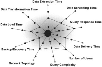
Figure 16-1: Data Warehouse Performance Characteristics.

The center of the chart in Figure 16-1 is the most desirable situation. The intersection at all dimensions indicates a practical or "implementable" state. Most dimensions are time sensitive. The closer you get to the center, the less time it takes to complete that task. When thinking of SAP BW performance, be creative to find ways to reduce time for one or more dimensions to optimize the overall performance.

For example, data extraction takes too much time due to extremely high transaction volume in SAP R/3. To handle this situation, you may decide to pull data from SAP R/3 multiple times a day instead of once a day. Keep this data in ODS in SAP BW and load data InfoCubes only once a day. If this option does not work for you, you may add additional processors in the SAP R/3 OLTP database server or add a dedicated application against an SAP R/3 instance to process data extracts quickly. The last two options could be expensive because they involve purchasing additional hardware.

Network bandwidth is another key factor in overall data warehouse performance. End-user queries receive large data volumes compared to OLTP transactions. Within a corporate Local Area Network (LAN) environment, end users may not feel much impact on the delivery of query results. However, Wide Area Network (WAN) and especially Internet users will experience poor information-delivery response time. To handle this network latency, SAP BW can be architected in data mart fashion to limit WAN data traffic or define queries that filter data at the SAP BW server level and return only a limited data set.

Optimizing Data Loads in SAP BW

Reducing data loads in BW is another major factor in improving overall data warehouse performance. Data loading in SAP BW is a complex process. Several factors contribute to performance factors; the following guidelines will improve data load time.

• Always load master data first. The SID tables are created at the time of master data load. When you load data in InfoCubes, all relevant SIDs needed to link dimensions and master tables are done for you. This reduces additional time needed to create SIDs during transaction data loads to populate InfoCubes.

• Drop the secondary indexes on the fact tables. Do not drop the primary key.

• Load data in ODS first, and then load data from ODS in the InfoCubes. The ODS here refers to the ODS in SAP BW 1.2B or the PSA in SAP BW 2.0.

• Rebuild the indexes on the fact table.

• Update the database statistics for cardinality information needed for the query optimizer to best query the execution path.

• Change the buffering of the Number Range Objects.

• Adjust IDOC-related parameters.

• Sort data to be loaded.

• Load data in parallel.

Remember, data warehouse performance is a balancing act. All of the previous items play a significant role in overall data load performance in SAP BW. Also note that only some of the data warehouse performance areas are specific to a DBMS used to implement SAP BW. The rest depends on SAP R/3 infrastructure, data models for the Information Objects (InfoCubes, ODS, Aggregate Cubes), and the queries. All such areas have to be regularly tuned for high-performance SAP BW implementation. Figure 16-2 shows how to set up InfoCube performance parameters in SAP BW 1.2B and SAP BW 2.0A.

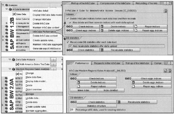
Figure 16-2: Setting up Data Load Performance Parameters in SAP BW 1.2B and SAP BW 2.0A.

Index Management

Prior to SAP BW release 1.2B, most index-related performance procedures were manual. However, in SAP BW 1.2B, these procedures are built into the InfoCube management options. Figure 16-2 shows how indexes are handled during InfoCube load time.

In the InfoCube tree, right-click an InfoCube and select the InfoCube Performance option. Then for SAP BW 1.2B, select InfoCube Performance; select Manage for SAP BW 2.0A. Check the Index Delete/Create options; the next time you load data, SAP BW will handle index deleting/re-creation automatically.

Buffering Number Range Objects

A Number Range object is like a Sequence Number in Oracle Database. It tracks the next available sequence number to assign to an associated object similar to a counter. Any time a new occurrence of the object is loaded in SAP BW, the system fetches the next sequence number value from the database, adds 1 to the current value, and saves it back in the database. When you are loading large amounts of data, you will do hundreds of extra database accesses to process sequence numbers, and that can be expensive.

To resolve this problem, you can buffer these sequencing objects in memory and set a range large enough that during data load, SAP BW simply obtains the next sequence number from memory instead of the database. This definitely improves overall data load performance.

Figure 16-3 shows how to set up Sequence Number buffering. To change the buffer for a Number Range object, run transaction SNRO and select the numbered buffer object name. Then from the Edit menu, select Set-up buffering and then select Main memory. Then in the Customizing specifications section, you will see that Main memory buffering is checked. Here you select your buffer range from 500 to 1,000.

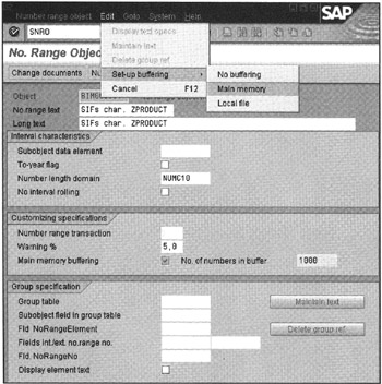
Figure 16-3: Changing Buffering of the Number Range Objects.

Caution 

Make sure that after you finish loading data, you change buffering back to the default setting.

InfoCube Aggregates

The size of any data warehouse grows rapidly in time and continues growing. It is not like an OLTP environment where you purge data to maintain a reasonable, manageable size for optimum transaction performance. A data warehouse is quite the opposite. You simply keep pumping data in the data warehouse, which needs constant monitoring of database growth and frequent database reorganizations.

Figure 16-4 shows the data growth pattern in a data warehouse. The reference data (master data) does increase, but volumes are often very low. The operational data-needed for warehouse administration such as sort areas, backup files, and temporary storage-remains almost the same. On the other hand, the analytical data such as InfoCubes, ODS, Aggregates, Query Results, and Documents grows almost exponentially. Note that data growth in a data warehouse is not continuous but in intervals; for example, toward the end of a quarter or month or at the end of the week, large transaction data sets are loaded and aggregated in a data warehouse. Similarly, data warehouse usage patterns vary from time to time and in intensity. For example, business profitability analysis activity is high just before the end of a month, quarter, or year, but senior executives want to review the past week's business operation every Monday morning for product production tactical planning. A good understanding of growth patterns and Information Objects usage helps database administrators to plan activities, such as database tuning and adding data files, before data loads start to fail.

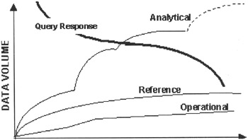
Figure 16-4: A Data Warehouse Data Volume Growth Pattern.

Tip 

Always plan for plenty of extra disk storage. Typically, the size of a data warehouse tends to be 4 to 10 percent larger than the actual transaction data.

As the size of an InfoCube grows, the query response starts to degrade, as shown in Figure 16-4. However, based on individual queries, one can define an aggregate cube, a view against an entire InfoCube based on a query definition. Aggregates are transparent to the end user. When a user or developer plans to design a query, only the InfoCube is visible to the end user in the BEX Analyzer. When a query is issued against an InfoCube, the OLAP processor determines which aggregate, if any, to use to quickly fetch the requested data.

In simple terms, an aggregate is a subset of an InfoCube based on a selected dimension value(s). For example, you have a sales analysis InfoCube that has four dimensions: Geography, Customer, Material, and Time. Suppose most of the sales analysis is done by Sales Regions (North America, Europe, South America, Africa, and Asia). Here you can build aggregates against the sales analysis InfoCube based on individual sales region, each having its own fact table and selected dimensions, containing sales information specific to the sales region.

When you issue a query against the sales analysis InfoCube, the OLAP optimizer will determine which aggregate to use to quickly retrieve data instead of searching through the entire sales InfoCube. Under this scenario, the aggregates are similar to dependent data marts as discussed in Chapter 1. Though aggregates are ideal for quick data access, they do impact data load times because now you have to update aggregates along with the InfoCubes. Therefore, do not define aggregates for all queries and frequently monitor their usage to qualify if you need one. Note that it is up to the SAP BW administrator to decide when to roll up aggregates after data loads in the InfoCubes to meet end-user data analysis needs.

The following steps are needed to define aggregates against an InfoCube to meet specific query data needs:

1. Identify end users' queries and their data navigation schemes

2. Identify fields to include in an aggregate

3. Identify field aggregate values

4. Identify filters to select specific data sets

5. Identify the hierarchy level

6. Define the aggregate

7. Activate the aggregate

8. Fill the aggregate with data (done automatically in BW 2.0)

Assume that the customer InfoCube is very large and queries are timing out. You may improve query responses by defining a few aggregate cubes. Look at the query definition. Identify which fields are used in each query. Do queries have built-in filters or restricted key figures? How do they use hierarchies? Do they start at a certain hierachy level? With this information, you will define InfoCubes that best meet end-user query needs.

Defining InfoCube Aggregates

To define aggregates, right-click the InfoCube, as shown in Figure 16-5, and select Maintain InfoCube aggregates.

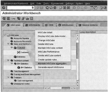
Figure 16-5: Defining Aggregates against the Customer InfoCube.

The Aggregate Maintenance window, displayed in Figure 16-6, shows an aggregate proposal based on queries defined against the Customer (0SD_C01) InfoCube. Initially, this is a blank screen.

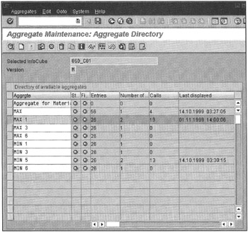
Figure 16-6: Defining Aggregates for an InfoCube in SAP BW 1.2B. Initially, When an Aggregate is Created, the Entries in the Calls and Last Displayed Columns are Not Filled in. as Users Use Queries against the InfoCube, SAP BW Automatically Fills Information About Each Aggregate on How Often and When an Aggregate was Used. Never-Used Aggregates Should be Deleted.

If you want to create aggregates based on present queries against the InfoCube, click the Simulate icon. The system analyzes all queries for the InfoCube and recommends one or more aggregates, as shown in Figure 16-6. Double-click an aggregate to edit or view its definition, as shown in Figure 16-7.

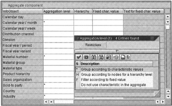
Figure 16-7: Defining Aggregates Selection Criteria in SAP BW 1.2B. Here You Select the Characteristics You Want to Include in the Aggregate. This Shows the Characteristics Selected for Aggregate MAX 1 for Customer InfoCube (0SD_C01).

Next, activate the aggregate and then click the Fill icon to load data from the aggregate cube from its InfoCube.

If you want to create a new aggregate manually in addition to what the system has proposed to you, click the New icon. You are then asked to specify the aggregate criterion. The rest of the process is the same.

The process of defining aggregates is quite similar to what it was in SAP BW 1.2B (see Figure 16-8). Here, aggregate activation and population of aggregates is done in one step when you activate the aggregate. Now you have the option of which type of aggregate proposal you want to use to define aggregates. In SAP BW 2.0, you have several choices: aggregate proposals from existing queries, from last navigation steps, BW statistics (from a database), or BW statistics (from an InfoCube).

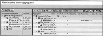
Figure 16-8: Defining Aggregates in SAP BW 2.0. In this Scenario, the Aggregate is Defined for a Specific Product, BIGSCREENTV, because End Users Want to do Extensive Sales Analysis for Large-Screen TVs.

After going through all this to define aggregates, you'd like to know how often they are going to be used. You need to know this to make decisions about which aggregates to drop. First, let end users run their queries to collect information on InfoCube and Aggregate usage. To find aggregate usage, simply launch the aggregate session. SAP BW will display when each aggregate was last used and the number of times it has been accessed in total. Figure 16-9 shows aggregate usage statistics for another SD cube I used to perform high-volume testing. The first aggregate has never been used; therefore, it is a prime target for deletion.

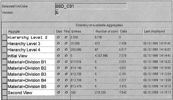
Figure 16-9: Aggregate Usage Statistics.

Aggregate cubes definitely improve query performance. The downside is that it takes longer to load data in InfoCubes. You have to be very careful about when to load data in InfoCubes and when to roll up aggregates to avoid any data inconsistency. Moreover, if you change master data, hierarchies, or navigational data, you should refresh (change run) the aggregates that could be time consuming depending on how many aggregates you have. Keep a close watch on the numbers in the Entries column (Figures 16-6 and 16-9). If the number of entries for a specific aggregate cube is less than 10 percent of the fact table, drop that aggregate because it will take more time and resources to build the aggregate as opposed to enhancing query performance.

---

Team-Fly