Data Flow Task Under the Hood

Any discussion about tuning the Data Flow Task necessarily starts from the Data Flow Task internals. To truly understand what's happening with data flow performance, you should be familiar with some important data flow concepts.

General Concepts

The Data Flow Task is actually a combination of various subsystems that interact through interfaces. Each subsystem is responsible for managing different aspects of the data flow behavior and is categorized into design time and execution time features. This chapter focuses on the execution time features because they have the most impact upon the performance of the data flow. Figure 23.1 shows a high-level system view of the Data Flow Task.

Figure 23.1. Data Flow Task system view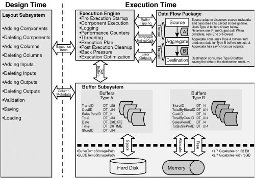

As you can see, there are four major components of interest to this discussion, as follows:

• Layout Subsystem Interacts with the designer and components to provide the design time configuration experience.

• Buffers Contain the data as it flows from the source to the destination.

• Buffer Subsystem Manages memory allocation, buffer creation, and spooling.

• Execution Engine Manages buffer "movement," execution planning, threads, and component calls. In short, this is Data Flow Task execution central, where it all comes together.

Layout Subsystem

The Layout Subsystem is the design time logic for the Data Flow Task. When you create a data flow in the designer, you are using this subsystem. Layout communicates with the Execution Engine and Buffer Subsystem by providing descriptions of the data flow from which the Execution Engine can build execution trees and the Buffer Subsystem can build buffers.

Buffers

Buffers are objects with associated chunks of memory that contain the data to be transformed. As data flows through the Data Flow Task, it lives in a buffer from the time that the source adapter reads it until the time that the destination adapter writes it. Generally speaking, data flow components use buffers for all their major memory needs, including privately created buffers for internal processing. Buffer objects contain pointers to column offsets and methods for accessing their memory chunks. The size and shape of a buffer is determined by several factors:

• Source metadata

• DefaultBufferMaxRows property on Data Flow Task

• DefaultBufferSize property on Data Flow Task

• MaxBufferSize/MinBufferSize internal values

• Buffer width

Source Metadata

If you've worked with the Data Flow Task at all, you're probably aware that it is very metadata dependent. In other words, it generally requires a connection to a server, flat file, or other source before you can start building the data flow. The origin of this metadata dependence is the buffer.

Note

One of the reasons the Data Flow Task is so fast is because there is little type ambiguity in the buffer, so very little memory is wasted on unused allocated buffer space and there is little pointer math needed to access a given cell in a buffer. Some users have decried the tight binding between metadata and the data flow because they would like to build more dynamic data flows that adjust to the metadata of the source on the fly. Although there have been long discussions about the legitimacy and value of such a feature, it is clear that the Data Flow Task was designed for optimal loading of big data and dynamically configuring itself to changing metadata was not within the original design goals. Perhaps, in future versions it will be added.

Figure 23.2 shows a simplistic representation of the structure of a buffer in memory.

Figure 23.2. Data flow buffer system view

Note the correspondence between the source or output column metadata types and the data column types in the buffer memory. Also note the row starts list. There is more to a buffer than the diagram shows, of course. The point to understand is that, on a simple level, the Data Flow Task is allocating memory to hold data and that components have access to the memory through methods provided on the buffer object.

DefaultBufferMaxRows

This setting controls the maximum allowable number of rows in a buffer and defaults to 10,000.

DefaultBufferSize

This is the default size of the buffer in bytes. The default is 10MB.

MaxBufferSize

This setting is internal and cannot be changed by the user and is the maximum allowable size for a buffer in bytes. In the release version of Integration Services 2005, this value was set to 100MB. The Data Flow Task will refuse to create buffers any larger than this to prevent wasting memory on empty buffers. If you attempt to increase DefaultMaxBufferSize to a value greater than MaxBufferSize, you will get an error similar to the following:

Could not set the property value: Error at Data Flow Task [DTS.Pipeline]: The default buffer size must be between 1048576 and 104857600 bytes. An attempt was made to set the DefaultBufferSize property to a value that is too small or too large.

MinBufferSize

This setting is the minimum allowable size of the buffer. By default, this value is the same as the allocation granularity for memory pages, usually 64K. The reason for this minimum is that memory operations are more efficient when memory is allocated in sizes with granularity the same as the virtual memory page size.

Buffer Width

The buffer width is the total number of bytes required to hold a row plus alignment adjustments. The row width is the sum of the widths of data types for all columns in the row. A row with two 8-byte integers (16), a 25-character Unicode string (50), and a Boolean (2) will be 68 bytes wide. The actual in-memory buffer row width might be wider than the actual data row width if the data row width does not align with the machine word boundary or if the buffer will contain copied columns.

Putting the Buffer Settings Together

The Data Flow Task only takes the MaxBuffer property values as suggestions and attempts to match those settings as well as can be done without compromising the performance of the data flow. Also, buffers are rarely exactly the same size as described by the properties because of various memory requirements, such as VirtualAlloc page allocation granularity and the need to align allocated memory structures on machine word boundaries.

Given these settings and their defaults, there are a few things you already know about the size and shape of buffers. First, buffers have a maximum size of 100MB and a minimum size of 64KB. By default, the buffers are 10MB in size and have no more than 10,000 rows per buffer. That much is clear.

What happens if the settings conflict? For example, if the size of a buffer (BufferWidth * DefaultMaxBufferRows) exceeds the DefaultMaxBufferSize setting? The Buffer Subsystem decreases the number of rows per buffer. What if the size of a buffer is less than MinBufferSize? The Buffer Subsystem increases the number of rows per buffer to meet the MinBufferSize setting. If the buffer size is between the minimum and maximum buffer size settings, the Buffer Subsystem attempts to allocate memory so as to match the number of rows requested. Generally speaking, the number of rows setting yields to the buffer size setting and is always rounded to page granularity.

Buffer Subsystem

The Buffer Subsystem manages memory for the Data Flow Task. It communicates with the Layout Subsystem to determine the shape of buffers, allocates memory, generates buffer types, creates and deletes buffers, detects low memory conditions, and responds to low memory conditions by spooling to disk if necessary. It also communicates with the Layout Subsystem to discover metadata and build appropriate buffer types to hold data rows during execution.

Execution Engine

The Execution Engine is at the heart of the data flow execution time behavior. It creates threads, plans executions, calls the various methods on components at the appropriate time and on the appropriate threads, logs output, and handles errors.

To graphically illustrate how the Execution Engine plans the work it will do, Figure 23.3 shows the Aggregate.dtsx package from the S19-StockComponents sample solution with the component, input, and output IDs added to the names.

Figure 23.3. A data flow annotated with the object IDs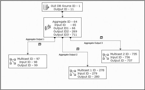

Note

Every object in the data flow is assigned an ID that is unique within the scope of the Data Flow Task. These IDs are how the Data Flow Task internally references all objects, including components, columns, inputs, and outputs.

Adding the input and output IDs in this manner is not something you would typically do, but it helps make the connection between the package data flow and the output the Execution Engine produces.

The data flow itself is very simplistic but ideal because, even though it is quite simple, it produces a fairly interesting and representative execution plan and execution trees and will be instrumental for exploring Execution Engine planning.

Execution Plans

At execution time, one of the first things the Execution Engine does is get the layout information from the Layout Subsystem. This is all the information about inputs, outputs, columns, sources, transforms, and destinations. Then, it builds an execution plan, which is essentially a list of operation codes, or opcodes for short. Each opcode represents a certain operation that the Execution Engine must perform.

Note

The Execution Engine logs the execution plan only if you have logging and the PipelineExecutionPlan log event enabled. To see the execution plan in the designer, open the Log Events window by right-clicking on the package design surface and selecting the Log Events menu option.

Figure 23.4 shows the execution plan for the sample package as viewed in the Log Entry dialog box. To open this dialog box, double-click on any log event in the Log Event window.

Figure 23.4. The execution plan shows the opcodes for the data flow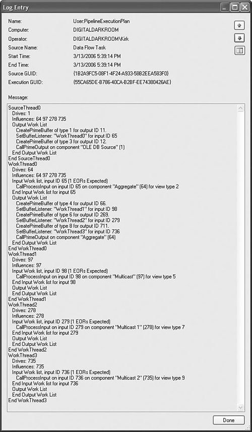

There is a lot of information provided in the execution plan and it can be a little confusing at times. However, if you take a little time to understand execution plans, you'll learn a lot about the internals of the Execution Engine. Walk through the plan starting from the top.

The "SourceThread0" Entry There are three types of threads in the Execution Engine:

• Administrative threads

• Source threads

• Worker threads

Administrative threads are hidden from you. They are the threads that do all the Execution Engine management. Although they are extremely important to the inner workings of the Execution Engine, they are never exposed to the user in the execution plan, and so forth. They are mentioned here simply as a point of interest.

Source threads, as their name implies, are created exclusively for the outputs of sources. When the Execution Engine is ready to have the source adapters start filling buffers with data, it calls the source adapter's PrimeOutput method on the source thread. The PrimeOutput calls on source adapters blocks. In other words, the call does not return until the source adapter is finished adding rows to the buffer provided in the PrimeOutput call.

Worker threads are used for everything else.

The "Drives: 1"

Entry The drives entry lists the components that the given thread drives. In this case, SourceThread0 drives the component with the ID of 1, or the OLE DB Source. What this means is that the methods of the listed components are called from the thread. So, if you look down the execution plan to the other "Drives" entries, and then compare the ID listed with the view of the data flow in Figure 23.3, you can quickly see which components are "driven" by which thread. WorkerThread0 drives the Aggregate with ID 64. WorkerThread1 drives Multicast with the ID 97, and so forth.

The "Influences"

Entry The influences list contains the IDs of those components that are impacted by the work done on the given thread. In this case, all the downstream components are influenced by SourceThread0 because it is such a simple data flow graph. However, this is not always the case and will definitely not be the case for separate data flow graphs within the same Data Flow Task.

Output Work List

The output work list is the set of opcodes that need to be executed on the given thread. For example, the output work list for SourceThread0 contains the following steps:

1.	CreatePrimeBuffer of type 1 for output ID 11Create a new buffer for output 11, which is the output for the OLE DB Source Adapter.
2.	SetBufferListener: "WorkThread0" for input ID 65Create a new thread to handle the input from the source. Input ID is the Aggregate input.
3.	CreatePrimeBuffer for output ID 12This is the error output for the OLE DB Source.
4.	CallPrimeOutput on Component "OLE DB Source"(1)This is the method call that kicks off the data flow execution and is the blocking call to the source for retrieving the data into the buffers.

You should be able to read the rest of the execution plan now because the rest of the entries are very similar to the SourceThread0 entry. By matching the execution plan entries and opcodes with the IDs in the package, you can see exactly what work the Execution Engine plans to do on each thread.

Execution Trees

Execution trees are where the output type, buffers, and threads come together to create opportunities for tuning the data flow. To see the execution tree output for a given package, enable the PipelineExecutionTrees log event. This log entry is similar to the execution plan log entry but a bit scaled down and only shows the relationship between the outputs and inputs in the data flow. As you'll see later in this chapter, execution trees can greatly impact data flow performance. Figure 23.5 shows the execution trees for the sample data flow in Figure 23.3.

Figure 23.5. The execution trees' output shows each thread's inputs and outputs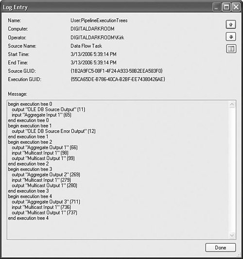

The execution trees for the sample package are trivial because it's such a simple package, but execution tree size has no theoretical limits and in practice can contain anywhere from one to tens of output/input pairings.

Although it's fairly easy to look at the execution trees' log output and see where each execution tree is on the data flow, it isn't so easy to understand how the execution trees are defined. A review of output types is in order.

Synchronous Outputs

You will recall that synchronous outputs for a given component use the same buffer type as one of the transforms inputs. Transforms with synchronous outputs generally do not copy memory, but rather modify the data within the buffer where it resides and process each buffer row by row in the order in which they arrive on the input. Synchronous outputs can add additional columns to the input buffers. If they do, the columns will exist on the buffer even before needed. For example, an execution tree containing a Derived Column transform will have additional columns in the buffer for the additional column or columns generated by the Derived Column transform and will only be visible to the Derived Column transform and all that follow it. Another way you can tell if an output is synchronous is it will have a nonzero value for its SynchronousInputID property. Asynchronous outputs have zero for this property value.

Asynchronous Outputs

Also recall that asynchronous outputs copy memory because they populate buffers of a different type than any of the inputs of the same component. There are two factors that cause an output to be asynchronous:

• The output creates data for a new buffer type. For example, the aggregate might release data from its outputs that doesn't remotely resemble the data on any of its inputs.

• The output does not release data at the same rate or in the same order as it appears on its associated input. For example, the Sort transform output buffers have the same metadata, but the inbound rows are all retained until the last one and then the sorted output is released from the transform.

Execution Tree Definitions

Depending on whom you ask, you'll get different definitions of what constitutes an execution tree because there is a lot of confusion about it and an individual must have a pretty good understanding of the Data Flow Task internals to understand the definition. You now have all the information you need to understand what an execution tree is.

An execution tree is a section of data flow starting from an asynchronous output and terminating at inputs on transforms that have no synchronous outputs. Some examples might help to clarify the concept.

Source Derived Column Data Conversion Sort Destination

Ignoring error outputs, the preceding data flow has two execution trees. Sources are always asynchronous because there is no input for the output. The Derived Column has synchronous outputs as well as the Data Conversion transform. However the Sort has asynchronous outputs and, so, the first execution tree starts at the Source output and ends at the Sort input. The second execution tree starts at the Sort output and ends at the Destination.

Here's another example:

Source1->Sort1 \                               |---> Merge ->Aggregate->Destination Source2->Sort2 / 

In the preceding data flow, there are exactly six execution trees.

• Source1 Output Sort1 Input

• Sort2 Input

• Merge Input

• Merge Input

• Aggregate Input

• Destination

Another way to think about execution trees is what they share in common. With the exception of those including sources, which have their own dedicated thread, transforms on the same execution tree share the same execution thread. They also share the same buffer type. However, as you'll soon discover, all the columns on a buffer are not always visible to all transforms on the same execution tree.

So, why does it matter? Why all this energy to describe execution trees? As it turns out, execution trees are an important concept to understand when tuning data flows. Execution trees are revisited later in this chapter in the "Turnkey Settings for Speedup" section.

Engine Threads

Engine threads are almost synonymous with execution trees. In the data flow shown previously, there are six threads, plus one thread that the runtime provides to the Data Flow Task. Remember that source threads block, so they are exclusively dedicated to the processing of sources. There is generally one thread for every execution tree. The formula for estimating threads needed for a given data flow is as follows:

number of threads = sources + execution trees

Understanding the threading is helpful when tuning data flows to more fully utilize a machine's available resources.

That's a quick primer on the Data Flow Task internals. There is a lot more, of course. This discussion just scratched the surface. You could write a whole book just about the Data Flow Task and someone probably will. However, what is covered here should be sufficient to understand the following discussions about how to tune your data flows.