Using the Business Intelligence Development Studio

The Business Intelligence Development Studio is the development platform for designing your Analysis Services databases. To start Business Intelligence Development Studio, click the windows Start button and go to Programs Microsoft SQL Server Business Intelligence Development Studio. If you're familiar with Visual Studio you might be thinking that the Business Intelligence Development Studio (BIDS) looks a lot like the Visual Studio environment. You're right; in Analysis Services 2005 you create Analysis Services projects in an environment that is essentially an augmented Visual Studio project environment. Working in the Visual Studio environment offers many benefits, such as easy access to source control and having many projects within the same Visual Studio solution (a solution within Visual Studio is a collection of projects such as Analysis Services project, C# project, Integration Services project or Reporting Services project).

Creating a Project in the Business Intelligence Development Studio

To design your Analysis Services database you need to create a project using BIDS. Typically you will design your database within BIDS, make appropriate design changes, and finally send the designed databases to your Analysis Services instance. Each project within BIDS becomes a database on an Analysis Services instance when all the definitions within the project are sent to the server. BIDS also provides you the option to directly connect to an Analysis Services database and make refinements to the database. Follow the steps below to create a new project.

To start BIDS, click the Start button and go to Programs Microsoft SQL Server Business Intelligence Development Studio. When BIDS launches, select File New Project.

In the BIDS select File New Project. You will see the Business Intelligence Project templates as shown in Figure 2-11. Click the Analysis Services project template. Type AnalysisServices2005Tutorial as the project name and select the directory in which you want to create this project. Click OK to complete the window.

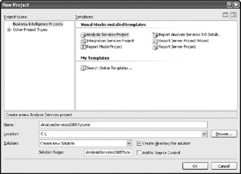
Figure 2-11

You are now in an Analysis Services project, as shown in Figure 2-12.

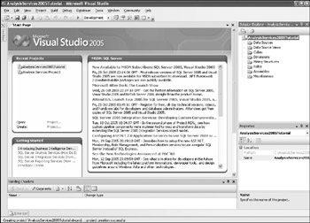
Figure 2-12

When you create a Business Intelligence project with a specific name, the project is automatically created under a solution with the same name. A solution will typically contain a collection of related projects. When you create a new project you have the option of adding the project to the existing solution or creating a new solution in the New Project dialog as shown in Figure 2-11. BIDS contains several panes; of most concern here are the Solution Explorer, Properties, and Output panes.

Solution Explorer Pane

The Solution Explorer pane in Figure 2-12 shows eight folders, each of which is described here:

• Data Sources. Your data warehouse is likely made up of disparate data sources such as Microsoft SQL Server, Oracle, DB2, and so forth. Analysis Services 2005 can easily deal with retrieving relational data from such configurations. Data sources are objects that contain details of a connection to a data source which include server name, login, password, etc. You establish connections to the relational servers by creating a data source for each one.

• Data Source Views. When working with a large operational data store you don't always want to see all the tables in the database; particularly while building an OLAP database using Analysis Services 2005. With Data Source Views (DSVs) you can limit the number of visible tables by including only the tables that are relevant to your analysis. DSVs help in creating a logical data model upon which you build your Unified Dimensional Model. A DSV can contain tables from one or more data sources, and one of these data sources is called a primary data source. Data sources and DSVs are discussed in Chapter 4.

• Cubes. Cubes are the foundation for analysis. A collection of measure groups (discussed later in this chapter) and a collection of dimensions form a cube. Each measure group is formed by a set of measures. Because cubes can have more than three dimensions, they are mathematical constructs and not necessarily three-dimensional cubes you can visually represent. You learn more about cubes later in this chapter and in Parts II and III.

• Dimensions. Dimensions are the categories by which you slice to view specific data of interest. Each dimension contains one or more hierarchies. Two types of hierarchies exist: the attribute hierarchy and user hierarchy. In this book, attribute hierarchies are referred to as attributes and user or multi-level hierarchies are referred to as hierarchies. Attributes correspond to columns of a dimension table, and hierarchies are formed by grouping several attributes. For example, most cubes have a Time dimension. A Time dimension typically contains the attributes Year, Month, Date, and Day and a hierarchy for Year-Month-Date. Sales cubes in particular often contain Geography dimensions, Customer dimensions, and Product dimensions. You learn about dimensions in Chapter 5.

• Mining Models. Data mining (covered in Chapter 13) is the process of analyzing raw data using algorithms that help discover interesting patterns not typically found by ad-hoc analysis. Mining Models are objects that hold information about a dataset after analysis by a specific algorithm which can be used for analyzing the patterns or predicting new data sets. Knowing these patterns can help companies make their business processes more powerful. For example, the book recommendation feature on http://www.Amazon.com relies on data mining.

• Roles. Roles are objects in a database that are used to control access permissions to the database objects (read, write, read/write, process) for users. If you want to provide only read access to a set of users you could create a single role that has read access and add all the users to this role. There can be several roles within a database. If a user is a member of several roles of a database, the user inherits the permissions of those roles. If there is a conflict in permissions, Analysis Services provides the most liberal access to the user. You learn more about roles in Chapters 12 and 19.

• Assemblies. Assemblies are user-defined functions that can be created by using a CLR language such as Visual Basic.NET, Visual C# .NET, or through languages such as Microsoft Visual Basic or Microsoft C++ that form Component Object Model (COM) binaries. These are typically used for custom operations that are needed for specific business logic and are executed on the server for efficiency and performance. Assemblies can be added at the server instance level or within a specific database. The scope of an assembly is limited to the object to which the assembly has been added. For example, if an assembly is added to the server, that assembly can be accessed within each database on the Server. On the other hand, if an assembly has been added within a specific database it can only be accessed within the context of that database. Within BIDS you can only add dot Net assembly references. You learn more about assemblies in Chapter 10.

• Miscellaneous. This object is used for adding any miscellaneous objects (design or meeting notes, queries, temporary deleted objects, and so on) that are relevant to the database project. These objects are stored in the project and are not sent to the Analysis Services instance when the database definition is created as a database on the Analysis Services instance.

Properties Pane

If you click an object in the Solution Explorer, the properties for that object appear in the Properties pane. Items that cannot be edited are grayed out. If you click a particular property, the description of that property appears in the Description pane at the bottom of the Properties pane.

Output Pane

The Output pane (to be seen later in this chapter) is used to report warnings and errors during builds. When a project is deployed to the server, progress reporting and error messages are displayed in this pane.

Creating an Analysis Services Database Using the Business Intelligence Development Studio

You are now ready to create a cube. The cube you create in this chapter is based on the relational database Adventure Works DW that ships with Microsoft SQL Server 2005. If SQL Server 2005 is installed on your machine with the sample databases, you will find the Adventure Works DW database on your machine. If you don't have SQL Server sample databases installed on your machine you can restore the database files (AdventureWorksDW.mdb, AdventureWorksDW.ldb). The Adventure Works DW files can be downloaded from the companion web site for this book.

Adventure Works DW contains sales information on a bicycle company. Figure 2-13 shows the structure of the data warehouse you build in this chapter, which consists of two fact tables and eight dimension tables. The fact table is highlighted at the top in the color yellow, and the dimension tables are highlighted in the color blue. The FactInternetSales and FactResellerSales are the fact tables. They contain several measures and foreign keys to the dimension tables. Both fact tables contain three dimension keys, ShipDateKey, OrderDateKey, and DueDateKey, that are joined to the dimension table DimTime. The FactInternetSales and the FactResellerSales fact tables join to the appropriate dimension tables by a single key as shown in Figure 2-13. The ParentEmployeeKey in the Employee table is joined with EmployeeKey in the same table which is modeled as a parent-child hierarchy. You learn parent-child hierarchies in Chapter 5.

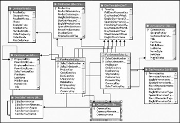
Figure 2-13

Create a Data Source

Cubes and dimensions of an Analysis Services database must retrieve their data values from tables in a relational data store. This data store, typically part of a data warehouse, must be defined as a data source. An OLE DB data provider or .NET data provider is used to retrieve the data from the data source. OLE DB and .NET data providers are industry standard technologies for retrieving data from relational databases. If your relational database provider does not provide a specific OLE DB data provider or a .NET data provider, you can use the generic Microsoft OLE DB provider to retrieve data. In this chapter you will be using the SQL Server database and hence you can use the OLE DB provider called Microsoft OLE DB Provider for SQL Server or the Native OLE DB\SQL Native Client provider. If you need to use the .Net data provider then you need to select SqlClient provider.

To create a data source, follow these steps:

1. Select the Data Sources folder in the Solution Explorer.

2. Right-click the Data Sources folder and then click New Data Source, as shown in Figure 2-14.

   
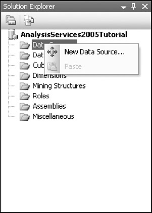
   Figure 2-14

   This launches the data source wizard. This wizard is self-explanatory and you can easily create a data source by making the appropriate selection on each page of the wizard. The first page of the wizard is the welcome page that provides additional information of a data source. Click Next to continue.

3. You're now in the connection definition page of the data source wizard, as shown in Figure 2-15. In this page you provide the connection information to the relational data source that contains the "Adventure Works DW" database. Click the New button under Data Connection Properties to specify the connection details. The Connection Manager Dialog box launches.

   
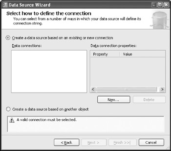
   Figure 2-15

4. On the page shown in Figure 2-16, you need to specify the connection properties to the SQL Server containing the Adventure Works DW database. The provider used to connect to any relational database by default points to Native OLE DB\SQL Native Client provider. Click on the drop down for the Provider and select Native OLEDB\SQL Native Client. or Microsoft OLE DB Provider for SQL Server. If you have installed SQL Server 2005 on the same machine, type localhost or the machine name under Server Name as shown in Figure 2-16. If you have restored the sample Adventure Works DW database on a different SQL Server machine, type that machine name instead. You can either choose Windows authentication or SQL Server Authentication for connecting to the relational data source. Select Use Windows Authentication. If you choose the SQL Server authentication you need to specify SQL Server login name and password. Make sure you check the Save my password option. Due to security restrictions in Analysis Services 2005, if you do not select this option you will be prompted to key in the password each time you send the definitions of your database to the Analysis Services instance. From the drop-down list box under Select or enter database name, select AdventureWorksDW. You have now provided all the details for establishing a connection to the relational data on Adventure Works DW. Click OK.

   
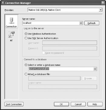
   Figure 2-16

5. The connection properties you provided in the connection dialog are now shown in the Select how to define the connection page of the Data Source wizard, as shown in Figure 2-17. Click the Next button.

   
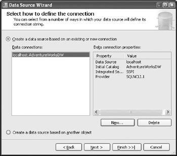
   Figure 2-17

6. In the Impersonation Information page you need to specify the impersonation details as to how Analysis Services will connect to the relational data source. There are four options for you to select as shown in Figure 2-18. You can provide a domain user name and password to impersonate or select the Analysis Service instance's service account for connection. If you choose the default option then the Analysis Services uses the impersonation information specified for the database. The option User the credentials of the current user is primarily used for data mining where you retrieve data from relational server for prediction. Select the Use the service account option and click Next.

   
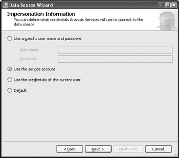
   Figure 2-18

7. On the final page, the Data Source wizard chooses the database you have selected as the name for the data source object you are creating (see Figure 2-19). You can choose the default name specified or specify a new name here. The connection string to be used for connecting to the relational data source is shown under Preview. Click Finish.

   
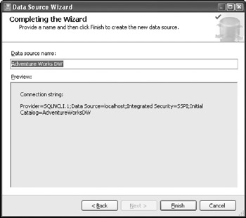
   Figure 2-19

Super! You have now successfully created a data source.

Create a Data Source View (DSV)

The Adventure Works DW database contains 25 tables. The cube you build in this chapter uses 10 tables. Data Source Views give you a logical view of the tables that will be used within your OLAP database. A Data Source View can contain tables and views from one or more data sources. Although you could accomplish the same functionality by creating views in the relational server, Data Source Views provide additional functionality, flexibility, and manageability.

To create a Data Source View, follow these steps:

1. Select Data Source Views folder in the Solution Explorer.

2. Right-click Data Source Views and select New Data Source View, as shown in Figure 2-20.

   
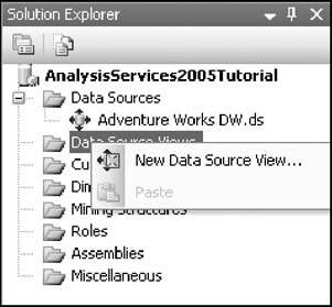
   Figure 2-20

   This launches the data source view wizard. Similar to the data source wizard, this wizard allows you to create a data source view just by choosing an appropriate selection on each page of the wizard. Click the Next button to go to the next page of the wizard.

3. The second page of the DSV wizard (see Figure 2-21) shows the list of data source objects from which you might want to create a view. The New Data Source button allows you to launch the data source wizard so that you can create new data source objects from the wizard. You have currently created a data source to the Adventure Works DW database. Select this data source and click the Next button.

   
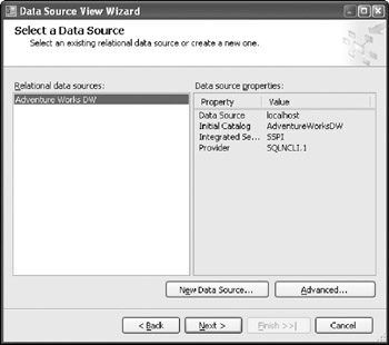
   Figure 2-21

4. Upon clicking the Next button, the DSV wizard connects to the relational database Adventure Works DW using the connection string contained in the data source object. The DSV then retrieves all the tables, views, and their relationships from the relational database and shows them in the third page. You can now select the tables and views that would be needed for the Analysis Services database. For this tutorial navigate through the Available Objects list and select the FactInternetSales and FactResellerSales tables. Click the > button so that the tables move to the Included Objects list. Select the two tables in the Included Objects list by holding down the Shift key. As soon as you select these tables you will notice that the Add Related Tables button is enabled. This button helps you to add all the tables and views that have relationships with the selected tables in the Included Objects list. Now click the Add Related Tables button. You will notice that all the related dimension tables mentioned earlier as well as the FactInternetSalesReason table are added to the Included Objects list. In this tutorial you will not be using the FactInternetSalesReason table, so you should remove this table. Select the FactInternetSalesReason table in the Included Objects list and click the < button. You have now selected all the tables needed to build the cube in this tutorial. Your Included Objects list of tables should match what's shown in Figure 2-22.

   
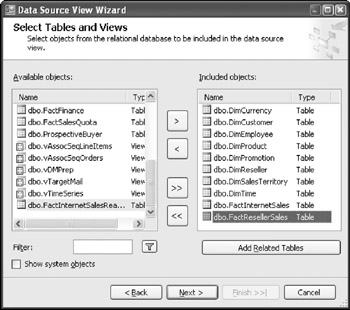
   Figure 2-22

5. Click the Next button and you are at the final page of the DSV Wizard! Similar to the final page of the data source wizard, you can specify your own name for the DSV object or use the default name. Select the default name presented in the wizard and click Finish.

You have now successfully created the DSV that will be used in this chapter. The DSV object is shown on the Solution Explorer with a new designer page created in the main area of the BIDS as shown in Figure 2-23. This is called the data source view editor. The data source view editor contains three main areas: diagram organizer, table view, and the diagram view. The Diagram view shows a graphical representation of the tables and their relationships. Each table is shown with all the columns of the table along with the key attribute. Connecting lines show the relationships between tables. If you double-click the connecting line you will find the columns of each table that are used to form the join. You can make changes to the data source view by adding, deleting, or modifying tables and views in the DSV Editor. In addition, you can establish new relationships between tables. You learn further details about the DSV Editor in Chapter 4.

Figure 2-23

The number of tables you can see in the Diagram view depends on the resolution on your machine. In this view, you can zoom in to see a specific table enlarged or zoom out to see all the tables within the Diagram view. To use the zoom feature you can right-click anywhere within the Diagram view, select Zoom, and set the zoom percentage you want. Figure 2-24 shows a zoomed in Diagram view so that you can see the FactInternetSales table clearly.

Figure 2-24

The Diagram view in the DSV arranges the tables to best fit within the view. Sometimes the number of tables in the DSV can be quite large. In such circumstances navigating to the tables in the Diagram view can be difficult. For easier navigation you can use the Locator window (see Figure 2-24). The Locator window shows the full DSV diagram as a thumbnail. You can open it by performing a left mouse click on the 4-headed arrow in the lower-right corner of the diagram, as highlighted in Figure 2-23. The Locator window remains open while the mouse button is held down. This allows you to navigate through the visible area in the diagram view by moving the mouse.

You have now learned the basic operations used within a data source view. Next, you move on to create the cube using cube wizard.

Create a Cube Using the Cube Wizard

In Analysis Services 2005 you can build cubes via two approaches — top-down or bottom-up. The traditional way of building cubes is bottom-up by building cubes from existing relational databases. In the bottom-up approach you need a data source view from which a cube can be built. Different cubes within a project can be built from a single DSV or from different DSVs. In the top-down approach you create the cube and then generate the relational schema based on the cube design.

A cube in Analysis Services 2005 consists of one or more measure groups from a fact table (typically you will have one measure group per fact table) and one or more dimensions (such as Product and Time) from the dimension tables. Measure groups consist of one or more measures (for example, sales, cost, count of objects sold). When you build a cube, you need to specify the fact and dimension tables you want to use. Each cube must contain at least one fact table, which determines the contents of the cube. The facts stored in the fact table are mapped as measures in a cube. Typically, measures from the same fact table are grouped together to form an object called measure group. If a cube is built from multiple fact tables, the cube typically contains multiple measure groups. Before building the cube the dimensions need to be created from the dimension tables. The cube wizard packages all the steps involved in creating a cube into a simple sequential process:

1. Launch the Cube Wizard by right-clicking the Cube folder in the Solution Explorer and selecting New Cube.

2. Click the Next button in the welcome page.

3. You are now asked to select the method to build the cube. Choose the default value and then click the Next button (see Figure 2-25). Note you are using the Cube Wizard.

   
   Figure 2-25

4. In the Select Data Source View page, select the Adventure Works DW DSV (see Figure 2-26) you created and click Next.

   
   Figure 2-26

5. The wizard will detect the relationships between the tables in the DSV and detects the fact and dimension tables. The next page of the Cube Wizard, Detecting Fact and Dimension Tables (see Figure 2-27), performs the analysis. Click the Next button after the wizard has completed the analysis.

   
   Figure 2-27

6. In the Identify Fact and Dimension Tables page (see Figure 2-28) the cube wizard presents you the fact and dimension tables from its analysis. If you feel the cube wizard's analysis does not match your design of fact and dimension tables you can make appropriate changes on this page so that the tables reflect the intended behavior for your design. In this example the cube wizard detects the DimReseller table as both fact and dimension table due to the relationships (outward relationship means fact table and inward relationship means dimension table) associated with the DimReseller table. Deselect the check box so that DimReseller is used as a dimension in this design as shown in Figure 2-28. Click Next to go to the next page.

   
   Figure 2-28

7. In the Select Measures page (see Figure 2-29), the cube wizard shows you the columns of the fact table that have been analyzed by the wizard as potential measures. The cube wizard has automatically removed the columns that join to the dimension tables because these columns are typically not used as measures. The cube wizard creates a measure group that has the same name as the fact table and groups all the measures under this measure group name. If there are multiple fact tables, the cube wizard groups the measures under appropriate measure groups. By default the cube wizard selects all the measures from the fact table. You have the option to select or de-select measures you want to be built in the cube. Select all the measures (by default all measures are selected) and click Next.

   
   Figure 2-29

8. The cube wizard now scans all the dimension tables to identify hierarchies within the dimension tables. The wizard samples the relational data from each dimension table, analyzes the relationships between columns within each dimensional table, and detects hierarchies. Each dimension contains one or more hierarchies. As mentioned earlier, two kinds of hierarchies are created within a dimension in Analysis Services 2005: attribute hierarchies and user hierarchies. Each column in a dimension table can be created as a flat hierarchy called the attribute hierarchy. Flat hierarchies are hierarchies that are formed from a single column in the dimension table. All the members of an Attribute hierarchy are at the lowest level. The attribute hierarchy also contains an All level (explained in Chapter 5). User hierarchies, on the other hand, are typically created with more than one level and are called multi-level hierarchies. A typical example of a user hierarchy is a geography hierarchy that contains the levels Country, State, City, and Zip Code. Each level in a user hierarchy typically corresponds to a column in the dimensional table. The Detecting Hierarchies page (see Figure 2-30) shows you the tables analyzed. Click Next to proceed to the next page.

   
   Figure 2-30

9. The Review New Dimensions page (see Figure 2-31) shows the dimensions that the wizard has detected. Here you can select or de-select the dimension you want the wizard to create based on the analysis. You can expand each dimension shown in this page to see the hierarchies detected by the wizard. The Attributes are shown under the Attributes folder and the Hierarchies are shown under the Hierarchies folder. After you have reviewed and selected the hierarchies and dimension, click Next.

   
   Figure 2-31

10. You are now in the last page of the wizard, as shown in Figure 2-32. Use the default name suggested by the wizard and click the Finish button.

    
    Figure 2-32

11. After the completion of the wizard you will notice that the cube Adventure Works DW and dimensions Dim Time, Dim Currency, Dim Customer, Dim Sales Territory, Dim Product, Dim Promotion, Dim Employee and Dim Reseller are created in the Solution Explorer as shown in Figure 2-33.

    
    Figure 2-33

    The cube Adventure Works DW in the Solution Explorer is automatically opened and that becomes your main window, called the Cube Editor, as shown in Figure 2-34.

    
    Figure 2-34

The cube editor has several panes that allow you to perform various operations that could be performed on a cube object. Your default pane upon completion of the cube wizard is the Cube Structure pane. Other panes of the Cube Editor are Dimension Usage, Calculation, KPIs, Actions, Partitions, Perspectives, Translations, and Browser. In this chapter you will become familiar with basic operations in the Cube Structure and the Browser panes. You learn more about the Cube Editor in Chapters 6 and 9.

The Cube Editor pane has been divided into three windows: Measures, Dimensions, and the Data Source View. If you need to add or modify Measure groups or Measures you will do that within the Measures window. The Dimensions window is used to add or modify the dimensions relevant to the current cube.

The Data Source View shows all the fact and dimension tables used in the cube with appropriate colors (yellow for fact table and blue for dimension table). Actions such as zoom in, zoom out, navigation, finding tables, and different diagram layouts of the tables that are possible in the DSV Editor are available within the DSV of the Cube Editor.

If you right-click within the Measure, Dimension, or Data Source View windows you will be able to see the various actions that could be accomplished within the windows. The actions within the Measure, Dimension, or DSV windows of a Cube Editor can also be accomplished by clicking the appropriate icons (see Figure 2-34) in the Cube Editor.

You have now successfully created a cube using the Business Intelligence Development Studio. All you have done, though, is create the structure of the cube. There has not been any interaction with the Analysis Services instance until this moment. This method of creating the cube structure without any interaction with the Analysis Services instance is referred to as project mode. Using BIDS you can also create these objects directly on the Analysis Services instance. The method of creating all the objects on the Server is called online mode, which is discussed in Chapter 9.

Next, you need to send the schema definitions of the newly created cube to the Analysis Services instance. This process is called deployment.

Deploying and Browsing a Cube

To deploy the database to the Analysis Server, right-click the project name and select Deploy, as shown in Figure 2-35. You can also deploy the project to the server from the menu items within BIDS by selecting the Debug Start or just by pressing the function key F5 on your keyboard.

Figure 2-35

When you select Deploy, the BIDS first builds the project you have created and checks for preliminary errors such as invalid definitions within the project. After that, BIDS packages all the objects and definitions you have created in the project and sends them to the Analysis Services instance. By default all these definitions are sent to Analysis Services on the same machine (localhost). A database with the name of the project is created in Analysis Services and all the objects created in the project will be created within this database. Upon selecting the Deploy option, BIDS not only sends all the schema definitions of the objects you have created, but also sends a command to process the database.

If you want to deploy this to a different machine that is running Analysis Services 2005, you need to right-click the project and select Properties. This brings up the Properties page in which you can specify the Analysis Services name to deploy the project. This page is shown in Figure 2-36. Change the Server property to the appropriate machine and follow the steps to deploy the project.

Figure 2-36

After you deploy the project you will see a Deployment Progress window at the location of the Properties window. The Output window in BIDS shows the operations that occur after selecting Deploy — building the project, deploying the definitions to the server, and the process command that is sent to the server. BIDS retrieves the objects being processed by the Analysis Services and shows the details (the object being processed; the relational query sent to the relational database to process that object including the start and end time; and errors, if any) in the Deployment Progress window. Once the deployment has been completed, then appropriate status will be shown in the Deployment Progress window as well as the Output window. If there were errors reported from the server these will be presented to you in the Output window. You can use the Deployment Progress window to identify which object caused the error. BIDS waits for results from the server. If the deployment succeeded (successful deployment of schema and processing of all the objects), this information is shown as "Deploy: 1 succeeded, 0 failed, 0 skipped." You will also notice the message "Deployment Completed Successfully" in the Deployment Progress window. If there are any errors reported from Analysis Services, then deployment will fail and you will be prompted with a dialog box. The errors returned from the service will be shown in the Output window. In your current project, deployment will succeed as shown in Figure 2-37 and you will be able to browse the cube.

Figure 2-37

After a successful deploy BIDS automatically switches the Cube Editor pane from Cube Structure to Browser so that you can start browsing the cube you have created. The Browser pane has three main windows, as shown in Figure 2-38. The left window shows all the measures and dimensions that are available for your browser. This is called the Metadata window. You can expand the tree structures to see the measure groups, measures, and hierarchies. On the right side you have two windows split horizontally. The top pane is referred to as the Filter window because you can specify filter conditions while browsing the cube. The bottom pane hosts the Office Web Components (OWC) inside it, which is used for analyzing results. You can drag and drop measures and dimensions from the metadata pane to the OWC in the right bottom pane to analyze data.

Figure 2-38

In Figure 2-38 you can see that the hierarchies "English Promotion Category" of dimension "Dim Promotion" and the hierarchy "Sales Territory Group" of dimension "Dim Sales Territory" are dropped on to the Column and Row fields of the OWC. Drag and drop the Measure Sales Amount in the Data area. You can similarly drag and drop multiple measures within the data area. You will now see the measure values that correspond to the intersection of the different values of the two hierarchies English Promotion Category and Sales Territory Group. As shown in Figure 2-38 you will notice "Grand Total" generated for each dimension along the Row and Column. This is provided by OWC and the values corresponding to the Grand Total are retrieved by OWC by sending appropriate MDX queries to the server. Each measure value corresponding to the intersection of the dimension values is referred to as a cell. If you hover over each cell you will see a window that shows all the properties of a particular cell. In Figure 2-87 you can also see the cell properties for the cell at the intersection of English Promotion Category = Reseller and Sales Territory Group = North America.