Key Elements of a Data Warehouse

Learning the elements of a data warehouse or data mart is, in part, about building a new vocabulary; the vocabulary associated with data warehousing can be less than intuitive, but once you get it, it all makes sense. The challenge, of course, is understanding it in the first place. Two kinds of tables form a data warehouse: fact tables and dimension tables.

Figure 1-3 shows a fact and a dimension table and the relationship between them. A fact table typically contains the business fact data such as sales amount, sales quantity, the number of customers, and the foreign keys to dimension tables. A foreign key is a field in a relational table that matches the primary key column of another table. Foreign keys provide a level of indirection between tables that enable you to cross-reference them. One important use of foreign keys is to maintain referential integrity (data integrity) within your database. Dimension tables contain detailed information relevant to specific attributes of the fact data, such as details of the product, customer attributes, store information, and so on. In Figure 1-3, the dimension table Product contains the information Product SKU and Product Name. The following sections go into more detail about fact and dimension tables.

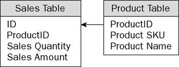
Figure 1-3

Fact Tables

With the end goal of extracting crucial business insights from your data, you will have to structure your data initially in such a way as to facilitate later numeric manipulation. Leaving the data embedded in some normalized database will never do! Your business data, often called detail data or fact data, goes in a de-normalized table called the fact table. Don't let the term "facts" throw you; it literally refers to the facts. In business, the facts are things such as number of products sold and amount received for products sold. Yet another way to describe this type of data is to call them measures. Calling the data measures versus detail data is not an important point. What is important is that this type of data is often numeric (though it could be of type string) and the values are quite often subject to aggregation (pre-calculating roll-ups of data over hierarchies, which subsequently yield improved query results). A fact table often contains columns like the ones shown in the following table:

Product ID	Date ID	State ID	Number of Cases	Sales Amount
1	07/01/2005	6	3244	$90,842
1	07/01/2005	33	6439	$184,000
1	07/01/2005	42	4784	$98,399
1	08/01/2005	31	6784	$176,384
1	08/01/2005	6	2097	$59,136
1	08/01/2005	33	7326	$8,635
1	08/01/2005	42	4925	$100,962
1	09/01/2005	31	8548	$176,384
1	09/01/2005	6	945	$26,649
1	09/01/2005	33	8635	$246,961
1	09/01/2005	42	4935	$101,165
1	10/01/2005	31	9284	$257,631
1	10/01/2005	33	9754	$278,965
1	10/01/2005	42	4987	$102,733
…	…	…	…	…

This table shows the sales of different varieties of beer between the months of July and October 2005 in four different states. The product id, date id, and state ids together form the primary key of the fact table. The number of cases of beer sold and the sales amount are facts. The product id, date id, and state id are foreign keys that join to the products, date, and state tables. In this table the state ids 6, 31, 33, and 42 refer to the states MA, CA, OR, and WA, respectively, and represent the order in which these states joined the United States. Building the fact table is an important step towards building your data warehouse.

Dimension Tables

The fact table typically holds quantitative data; for example, transaction data that shows number of units sold per sale and amount charged to the customer for the unit sold. To provide reference to higher-level roll-ups based on things like time, a complementary table can be added that provides linkage to those higher levels through the magic of the join (how you link one table to another). In the case of time, the fact table might only show the date on which some number of cases of beer was sold; to do business analysis at the monthly, quarterly, or yearly level, a time dimension is required. The following table shows what a beer products dimension table would minimally contain. The product id is the primary key in this table. The product id of the fact table shown previously is a foreign key that joins to the product id in the following table:

Product ID	Product SKU	Product Name
1	SBF767	SuperMicro Ale
2	SBH543	SuperMicro Lager
3	SBZ136	SuperMicro Pilsner
4	SBK345	SuperMicro Hefeweizen
…	…	…

For illustrative purposes, assume that you have a dimension table for time that contains monthly, quarterly, and yearly values. There must be a unique key for each value; these unique key values are called primary keys. Meanwhile, back in the fact table you have a column of keys with values mapping to the primary keys in the dimension table. These keys in the fact table are called foreign keys. For now it is enough if you get the idea that dimension tables connect to fact tables and this connectivity provides you with the ability to extend the usefulness of your low-level facts resident in the fact table.

A multi-dimensional database is created from fact and dimension tables to form objects called dimensions and cubes. Dimensions are objects that are created mostly from dimension tables. Some examples of dimensions are time, geography, and employee which would typically contain additional information about those objects by which users can analyze the fact data. The cube is an object that contains fact data as well as dimensions so that data analysis can be performed by slicing or dicing dimensions. For example, you could view the sales information for the year 2005 in the state of Washington. Each of those slices of information is a dimension.

Dimensions

To make sense of a cube, which is at the heart of business analysis and discussed in the next section, you must first understand the nature of dimensions. We say that OLAP is based on multidimensional databases because it quite literally is. You do business analysis by observing the relationships between dimensions like Time, Sales, Products, Customers, Employees, Geography, and Accounts. Dimensions are most often made up of several hierarchies. Hierarchies are logical entities by which a business user might want to analyze fact data. Each hierarchy can have one or more levels. A hierarchy in the geography dimension, for example, might have the following levels: Country, State, County, and City.

A hierarchy like the one in the geography dimension would provide a completely balanced hierarchy for the United States. Completely balanced hierarchy means that all leaf (end) nodes for cities would be an equal distance from the top level. Some hierarchies in dimensions can have an unbalanced distribution of leaf nodes relative to the top level. Such hierarchies are called unbalanced hierarchies. An organization chart is an obvious example of an unbalanced hierarchy. There are different depths to the chain of supervisor to employee; that is, the leaf nodes are different distances from the top-level node. For example, a general manager might have unit managers and an administrative assistant. A unit manager might have additional direct reports such as a dev and a test manager, while the administrative assistant would not have any direct reports. Some hierarchies are typically balanced but are missing a unique characteristic of some members in a level. Such hierarchies are called ragged hierarchies. An example of a ragged hierarchy is a geography hierarchy that contains the levels Country, State, and City. Within the Country USA you have State Washington and City Seattle. If you were to add the Country Greece and City Athens to this hierarchy, you would add them to the Country and City levels. However, there are no states in the Country Greece and hence member Athens is directly related to the Country Greece. A hierarchy in which the members descend to members in the lowest level with different paths is referred to as a ragged hierarchy. Figure 1-4 shows an example of a Time dimension with the hierarchy Time. In this example, Year, Quarter, Month, and Date are the levels of the hierarchy. The values 2005 and 2006 are members of the Year level. When a particular level is expanded (indicated by minus sign in the figure) you can see the members of the next level in the hierarchy chain.

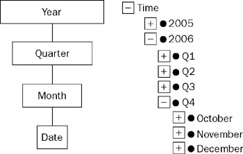
Figure 1-4

To sum up, a dimension is a hierarchical structure that has levels that may or may not be balanced. It has a subject matter of interest and is used as the basis for detailed business analysis.

Cubes

The cube is a multidimensional data structure from which you can query for business information. You build cubes out of your fact data and the dimensions. A cube can contain fact data from one or more fact tables and often contains a few dimensions. Any given cube usually has a dominant subject under analysis associated with it. For example, you might build a Sales cube with which you analyze sales by region, or a Call Processing cube with which you analyze length of call by problem category reported. These cubes are what you will be making available to your users for analysis.

Figure 1-5 shows a Beer Sales cube that was created from the fact table data shown previously. Consider the front face of the cube that shows numbers. This cube has three dimensions: Time, Product Line, and State where the product was sold. Each block of the cube is called a cell and is uniquely identified by a member in each dimension. For example, analyze the bottom-left corner cell that has the values 4,784 and $98,399. The values indicate the number of sales and the sales amount. This cell refers to the sales of Beer type Ale in the state of Washington (WA) for July 2005. This is represented as [WA, Ale, Jul '05]. Notice that some cells do not have any value; this is because no facts are available for those cells in the fact table.

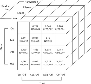
Figure 1-5

The whole point of making these cubes involves reducing the query response time for the information worker to extract knowledge from the data. To make that happen, cubes typically contain pre-calculated summary data called aggregations. Querying existing aggregated data is close to instantaneous compared to doing cold (no cache) queries with no pre-calculated summaries in place. This is really at the heart of business intelligence, the ability to query data with possibly gigabytes or terabytes of pre-summarized data behind it and yet get an instant response from the server. It is quite the thrill when you realize you have accomplished this feat!

You learned about how cubes provide the infrastructure for storing multidimensional data. Well, it doesn't just store multidimensional data from fact tables; it also stores something called aggregations of that data. A typical aggregation would be the summing of values up a hierarchy of a dimension. For example, summing of sales figures up from stores level, to district level, to regional level; when querying for those numbers you would get an instant response because the calculations would have already been done when the aggregations were formed. The fact data does not necessarily need to be aggregated as sum of the specific fact data. You can have other ways of aggregating the data such as counting the number of products sold. Again, this count would typically roll up through the hierarchy of a dimension.

The Star Schema

The entity relationship diagram representation of a relational database shows you a different animal altogether as compared to the OLAP (multidimensional) database. It is so different in fact, that there is a name for the types of schemas used to build OLAP databases: the star schema and the snowflake schema. The latter is largely a variation on the first. The main point of difference is the complexity of the schema; the OLTP schema tends to be dramatically more complex than the OLAP schema. Now that you know the infrastructure that goes into forming fact tables, dimension tables, and cubes, the concept of a star schema should offer little resistance. That is because when you configure a fact table with foreign key relationships to one or more of a dimension table's primary keys, as shown in Figure 1-6, you have a star schema. Looks a little like a star, right?

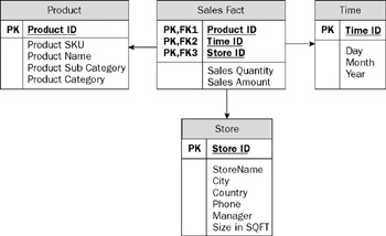
Figure 1-6

The star schema provides you with an illustration of the relationships between business entities in a clear and easy-to-understand fashion. Further, it enables number crunching of the measures in the fact table to progress at amazing speeds.

The Snowflake Schema

If you think the star schema is nifty, and it is, there is an extension of the concept called the snowflake schema. The snowflake schema is useful when one of your dimension tables starts looking as detailed as the fact table it is connected to. With the snowflake, a level is forked off from one of the dimension tables, so it is separated by one or more tables from the fact table. In Figure 1-7 the Product dimension has yielded a Product Category level. The Product Sub Category level is hence one table removed from the sales fact table. In turn, the Product Sub Category level yields a final level called the Product Category — which has two tables of separation between it and the sales fact table. These levels, which can be used to form a hierarchy in the dimension, do not make for faster processing or query response times, but they can keep a schema sensible.

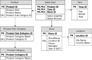
Figure 1-7

You have so far learned the fundamental elements of a data warehouse. The biggest challenge is to understand these well and design and implement your data warehouse to cater to your end-users. There are two main design techniques for implementing data warehouses. These are the Inmon approach and the Kimball approach.