Simple Linear Regression

---

In simple linear regression, there is a single quantitative independent variable. Suppose, for example, that you want to determine whether a linear relationship exists between the asking price for a house and its area in square feet. The area of the house is the quantitative independent variable, and the asking price for the house is the dependent variable.

The data set analyzed in this example is called Houses, and it contains the characteristics of fifteen houses for sale. The data set contains the following variables.

style	style category (ranch, split-level, condominium, or two-story)
sqfeet	area in square feet
bedrooms	Number of bedrooms
baths	Number of bathrooms
street	name of the street on which the house is located
price	asking price for the house

The task includes performing a simple regression analysis to predict the variable price from the explanatory variable, sqfeet.

Open the Houses Data Set

The data are provided in the Analyst Sample Library. To open the Houses data set, follow these steps:

1. Select Tools → Sample Data...

2. Select Houses.

3. Click OK to create the sample data set in your Sasuser directory.

4. Select File → Open By SAS Name...

5. Select Sasuser from the list of Libraries.

6. Select Houses from the list of members.

7. Click OK to bring the Houses data set into the data table.

Request the Simple Regression Analysis

To request the simple regression analysis, follow these steps:

1. Select Statistics → Regression → Simple...

2. Select price from the candidate list as the Dependent variable.

3. Select sqfeet from the candidate list as the Explanatory variable.

Figure 11.2 displays the resulting dialog.

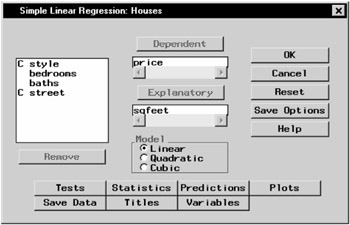
Figure 11.2: Simple Linear Regression Dialog

The model defined in this analysis is

• price = b₀ + b₁ sqfeet

If you select Quadratic or Cubic in the Model box, the respective model is

• price = b₀ + b₁ sqfeet + b₂ sqfeet²

or

• price = b₀ + b₁ sqfeet + b₂ sqfeet² + b₃ sqfeet³

The default analysis fits the simple regression model.

Request a Scatter Plot of the Data

To request a plot of the observed values versus the independent values, follow these steps.

1. Click on the Plots button.

2. Select Plot observed vs independent.

You can add 95% confidence limits for the mean of the independent variable by selecting Confidence limits, or you can produce 95% prediction limits for individual predictions.

3. Click OK.

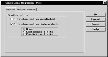
Figure 11.3: Simple Linear Regression— Plots Dialog

Click OK in the Simple Linear Regression dialog to perform the analysis.

Review the Results

The results are displayed in Figure 11.4. The ANOVA table is displayed in the results, followed by the table of parameter estimates. The least squares fit is

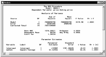
Figure 11.4: Simple Linear Regression— Results

• price = -14982 + 67.52 × sqfeet

The small p-values listed in the Pr > |t| column indicate that both parameter estimates are significantly different from zero.

The plot of the observed and independent variables is displayed in Figure 11.5. The plot includes the fitted regression line.

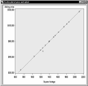
Figure 11.5: Simple Linear Regression— Scatter Plot with Regression Line

---