Getting Started

---

In this example, you bring data into the Analyst data table, perform a regression analysis, and see the results in the project tree.

Bring Up Analyst and Create a Sample Data Set

Select Solutions → Analysis → Analyst from the main SAS menu.

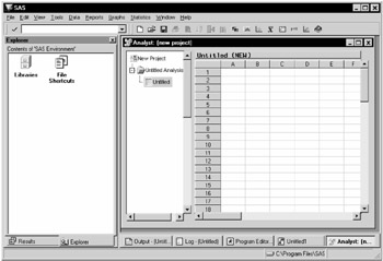
Figure 1.1: The Analyst Application with Explorer and Results Windows

You can close the Explorer and Results windows by clicking on the close box in the upper right corner of the windows. These windows are closed in the remaining examples in this book.

To use one of the sample data sets for this example, follow these steps:

1. Select Tools → Sample Data...

2. Select Fitness.

3. Click OK to create the sample data set in your Sasuser directory.

Bring the Data into the Data Table

To bring the sample data into the data table, follow these steps:

1. Select File → Open By SAS Name...

2. Select Sasuser from the list of Libraries.

3. Select Fitness from the list of members.

4. Click OK to bring the sample data into the data table.

When you bring the Fitness sample data into the data table, the Fitness Analysis folder, with a Fitness table node representing the data table, appears in the project tree.

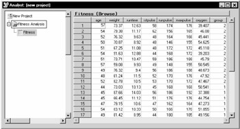
Figure 1.2: Fitness Analysis Folder in Project Tree

Perform a Regression Analysis

To run a simple linear regression on the Fitness data, follow these steps.

1. Select Statistics → Regression → Simple...to select the Simple Regression task.

2. In the Simple Linear Regression dialog, select oxygen from the list and click on the Dependent button to designate oxygen consumption as the dependent variable. Select runtime from the list and click on the Explanatory button to designate the amount of time to run 1.5 miles as the explanatory variable.

   
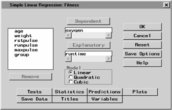
   Figure 1.3: Dependent and Explanatory Variables

3. To create a scatter plot of your results, click on the Plots button. In the Predicted tab, select Plot observed vs independent.

   
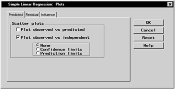
   Figure 1.4: Scatter Plot

   Click OK.

4. In the Simple Linear Regression dialog, click on the Titles button to specify a title for your results. In the first field of the Titles dialog, type Speed vs. Oxygen Consumed.

   
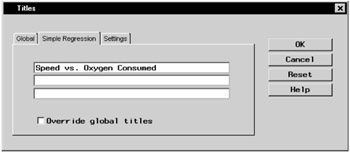
   Figure 1.5: Title

   Click OK.

5. Click OK in the Simple Linear Regression dialog to generate the results.

Your Results

When you click OK in the Simple Linear Regression dialog, the output from a simple linear regression is automatically displayed in the Analysis window. Drag the borders of the Analysis window until you can see all of the output.

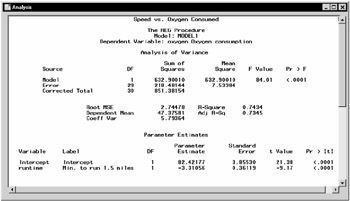
Figure 1.6: Simple Regression Output

This model might be considered minimally adequate with an R-square value of 0.7434; the negative coefficient for runtime indicates that the linear relationship between oxygen consumption and running time is a negative one.

You can save and print your results from this window. You can also copy your output to the Program Editor window, where you can copy it to the clipboard and paste it into other applications.

Close the Analysis window to see the project tree. In addition to output, a scatter plot and the SAS code used to perform the regression and create the scatter plot are displayed as nodes in the project tree by default.

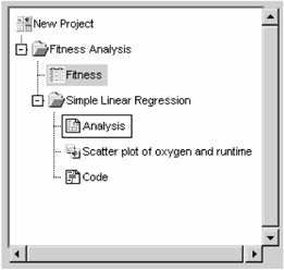
Figure 1.7: Results in Project Tree

Double-click on the Scatter plot node to view the scatter plot that you have created.

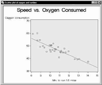
Figure 1.8: Scatter Plot

The scatter plot illustrates the results of your simple linear regression: higher oxygen consumption rates are associated with lower running times. You can change the graph to fit the window, edit the graph, or save it to a different format, such as GIF, by selecting File → Save As...

Close the Scatter Plot window to view the Code node in the project tree.

Double-click on the Code node to view the SAS code that was used to perform the simple linear regression and create the scatter plot.

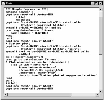
Figure 1.9: Code

Saving a Project

To save the project, follow these steps:

1. Select New Project at the top of the project tree.

2. Select Save...from the pop-up menu.

3. Type My Project in the Name: field.

   
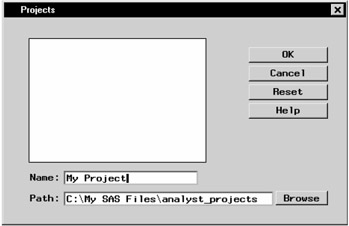
   Figure 1.10: Saving a Project

4. Click OK.

---