Chapter 10: Analysis of Variance

---

Introduction

Analysis of variance is a technique for exploring the variation of a continuous response variable (dependent variable). The response variable is measured at different levels of one or more classification variables (independent variables). The variation in the response due to the classification variables is computed, and you can test this variation against the residual error to determine the significance of the classification effects.

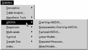
Figure 10.1: Analysis of Variance Menu

The Analyst Application provides several types of analyses of variance (ANOVA). The One-Way ANOVA task compares the means of the response variable over the groups defined by a single classification variable. See the section "One-Way Analysis of Variance" beginning on page 273 for more information.

The Nonparametric One-Way ANOVA task performs tests for location and scale differences over the groups defined by a single classification variable.

Eight nonparametric tests are offered. See the section "Nonparametric One-Way Analysis of Variance" beginning on page 279 for more information.

The Factorial ANOVA task compares the means of the response variable over the groups defined by one or more classification variables. This type of analysis is useful when you have multiple ways of classifying the response values. See the "Factorial Analysis of Variance" section beginning on page 284 for more information.

The Linear Models task enables you to compare means and explain variation when you have a model that includes classification variables, quantitative variables, or both (such as in an analysis of covariance). See the "Linear Models" section beginning on page 290 for more information.

You can use the Repeated Measures task when you have multiple measurements of the response variable for the same experimental unit over different times or conditions or when the response values are assumed to be correlated within certain groups. For detailed information, see Chapter 16, "Repeated Measures."

The Mixed Models task enables you to fit basic mixed models. A mixed model is a linear model that contains both fixed effects and random effects. For detailed information, see Chapter 15, "Mixed Models."

The examples in this chapter demonstrate how you can use the Analyst Application to perform one-way and factorial ANOVA as well as to fit the linear model.

The Air Quality Data Set

The data set used in the following examples contains measurements on air quality recorded in an industrial valley. The measurements are taken hourly for a period of one week.

The first variable in the data set Air is a SAS datetime variable (datetime) that contains the date and the time of day on which the observation was taken. The data set contains two additional time-related variables related to datetime that record the day of the week (day) and the hour of the day (hour).

The variables measuring air quality are co (carbon monoxide), o3 (ozone), so4 (sulfate), no (nitrous oxide), and dust (particulates). The final variable provided is wind, which gives the wind speed in knots.

Open the Air Data Set

The data are provided in the Analyst Sample Library. To access this Analyst sample data set, follow these steps:

1. Select Tools → Sample Data...

2. Select Air.

3. Click OK to create the sample data set in your Sasuser directory.

4. Select File → Open By SAS Name...

5. Select Sasuser from the list of Libraries.

6. Select Air from the list of members.

7. Click OK to bring the Air data set into the data table.

Create a New Variable

To perform the analyses in the following examples, you need to create a new variable to represent the factory workshift periods. The new character variable, shift, recodes the variable hour into three factory workshift periods. For information on recoding ranges and computing variables, see the section "Recoding Ranges" on page 44 in Chapter 2.

Figure 10.2 displays the Recoding Ranges Information dialog. Enter the information to create the new variable as shown in Figure 10.2.

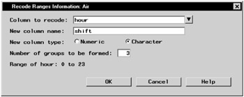
Figure 10.2: Recoding Ranges Information— Defining the New Variable

Click OK to display the Recoding Ranges dialog (Figure 10.3). To define the values for the new variable, shift, enter the values as shown in Figure 10.3.

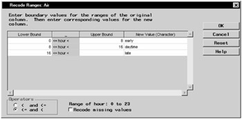
Figure 10.3: Recoding Ranges— Defining the Values for the New Variable

The values of the new variable shift are as follows: 'early' corresponds to the hours between 0 and 8 (from midnight until 8 a.m.), 'daytime' corresponds to the hours between 8 and 16 (from 8 a.m. until 4 p.m.), and 'late' corresponds to the hours greater than or equal to 16 (from 4 p.m. to midnight).

---