Producing One-Way Frequencies

---

The data set analyzed in the following sections is taken from the 1995 Statistical Abstract of the United States. The data are measures of the birth rate and infant mortality rate for 1992 in the United States. Information is provided for the 50 states and the District of Columbia. The states are grouped by region. Here, these data are considered to be a sample of yearly data.

Suppose you want to determine the frequency of occurrence of the various regions. In the following example, a listing of the frequencies and a bar chart are produced.

In the Frequency Counts task, you can compute one-way frequency tables for the variables in your data set. For each value of your analysis variable, Analyst produces the frequency, cumulative frequency, and cumulative percentage. You can control the order in which the values appear and specify group and count variables.

Open the Bthdth92 Data Set

The data are provided in the Analyst Sample Library. To open the Bthdth92 data set, follow these steps:

1. Select Tools → Sample Data...

2. Select Bthdth92.

3. Click OK to create the sample data set in your Sasuser directory.

4. Select File → Open By SAS Name...

5. Select Sasuser from the list of Libraries.

6. Select Bthdth92 from the list of members.

7. Click OK to bring the Bthdth92 data set into the data table.

Request Frequency Counts

To request frequency counts, follow these steps:

1. Select Statistics → Descriptive → Frequency Countsb

2. Select region as the frequencies variable from the candidate list.

The default analysis provides the information desired. Note that you can use the Input dialog to select the specific ordering by which the variable values are listed.

Figure 7.2 displays the Frequency Counts dialog with region specified as the frequencies variable.

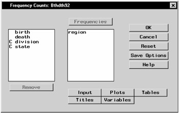
Figure 7.2: Frequency Counts Dialog

Request a Horizontal Bar Chart

To produce a horizontal bar chart in addition to the frequency counts, follow these steps:

1. Click on the Plots button.

2. Select Horizontal, as displayed in Figure 7.3.

   
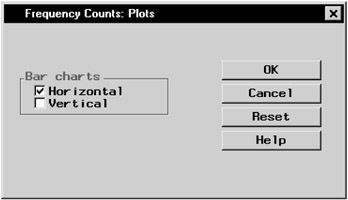
   Figure 7.3: Frequency Counts— Plots Dialog

3. Click OK to close the Plots dialog.

Click OK in the Frequency Counts main dialog to perform the analysis.

Review the Results

The results are presented in the project tree under the Frequency Counts folder, as displayed in Figure 7.4. The three nodes represent the frequency counts output, the horizontal bar chart, and the SAS programming statements (labeled Code) that generate the output.

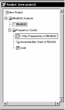
Figure 7.4: Frequency Counts— Project Tree

You can double-click on any node in the project tree to view the contents in a separate window. Note that the first output generated is displayed by default.

Figure 7.5 displays the table of frequency counts for the variable region.

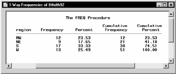
Figure 7.5: Frequency Counts— One-Way Frequencies of the Variable region

The table shows that about 33% of the observations in the data set are located in the southern region, and roughly 25% of the observations are located in the western and midwestern regions, respectively. Approximately 18% of the observations are located in the northeastern region.

To display the bar chart of the frequency counts, double-click the node labeled Horizontal Bar Chart of REGION (Figure 7.6).

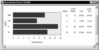
Figure 7.6: Frequency Counts— Horizontal Bar Chart by Region

---