Details

Input Data Set of Statistics

PROC TTEST accepts data containing either observation values or summary statistics. It assumes that the DATA= data set contains statistics if it contains a character variable with name _TYPE_ or _STAT_ . The TTEST procedure expects this character variable to contain the names of statistics. If both _TYPE_ and _STAT_ variables exist and are of type character, PROC TTEST expects _TYPE_ to contain the names of statistics including ˜N', ˜MEAN', and ˜STD' for each BY group (or for each class within each BY group for two-sample t tests). If no ˜N', ˜MEAN', or ˜STD' statistics exist, an error message is printed.

FREQ, WEIGHT, and PAIRED statements cannot be used with input data sets of statistics. BY, CLASS, and VAR statements are the same regardless of data set type. For paired comparisons, see the _DIF_ values for the _TYPE_ =T observations in output produced by the OUTSTATS= option in the PROC COMPARE statement (refer to the SAS Procedures Guide ).

Missing Values

An observation is omitted from the calculations if it has a missing value for either the CLASS variable, a PAIRED variable, or the variable to be tested . If more than one variable is listed in the VAR statement, a missing value in one variable does not eliminate the observation from the analysis of other nonmissing variables.

Computational Methods

The t Statistic

The form of the t statistic used varies with the type of test being performed.

• To compare an individual mean with a sample of size n to a value m , use

  

  where x is the sample mean of the observations and s ² is the sample variance of the observations.

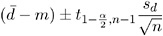
• To compare n paired differences to a value m , use

  

  where d is the sample mean of the paired differences and is the sample variance of the paired differences.

• To compare means from two independent samples with n ₁ and n ₂ observations to a value m , use

  

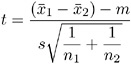
  where s ² is the pooled variance

  

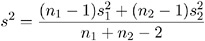
  and and are the sample variances of the two groups. The use of this t statistic depends on the assumption that = , where and are the population variances of the two groups.

The Folded Form F Statistic

The folded form of the F statistic, F ² , tests the hypothesis that the variances are equal, where

A test of F ² is a two-tailed F test because you do not specify which variance you expect to be larger. The p -value gives the probability of a greater F value under the null hypothesis that = .

The Approximate t Statistic

Under the assumption of unequal variances, the approximate t statistic is computed

where

The Cochran and Cox Approximation

The Cochran and Cox (1950) approximation of the probability level of the approximate t statistic is the value of p such that

where t ₁ and t ₂ are the critical values of the t distribution corresponding to a significance level of p and sample sizes of n ₁ and n ₂ , respectively. The number of degrees of freedom is undefined when n ₁ ‰  n ₂ . In general, the Cochran and Cox test tends to be conservative (Lee and Gurland 1975).

Satterthwaite's Approximation

The formula for Satterthwaite's (1946) approximation for the degrees of freedom for the approximate t statistic is:

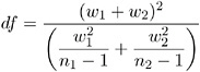
Refer to Steel and Torrie (1980) or Freund, Littell, and Spector (1986) for more information.

Confidence Interval Estimation

The form of the confidence interval varies with the statistic for which it is computed. In the following confidence intervals involving means, is the quantile of the t distribution with n ˆ’ 1 degrees of freedom. The confidence interval for

• an individual mean from a sample of size n compared to a value m is given by

  

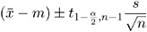
  where x is the sample mean of the observations and s ² is the sample variance of the observations

• paired differences with a sample of size n differences compared to a value m is given by

  

  where d and are the sample mean and sample variance of the paired differences, respectively

• the difference of two means from independent samples with n ₁ and n ₂ observations compared to a value m is given by

  

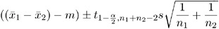
  where s ² is the pooled variance

  

  and where and are the sample variances of the two groups. The use of this confidence interval depends on the assumption that = , where and are the population variances of the two groups.

The distribution of the estimated standard deviation of a mean is not symmetric, so alternative methods of estimating confidence intervals are possible. PROC TTEST computes two estimates. For both methods, the data are assumed to have a normal distribution with mean µ and variance ƒ ² , both unknown. The methods are as follows :

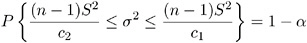
• The default method, an equal- tails confidence interval, puts an equal amount of area in each tail of the chi-square distribution. An equal tails test of H : ƒ = ƒ has acceptance region

  

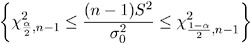
  which can be algebraically manipulated to give the following 100(1 ˆ’ ± )% confidence interval for ƒ ² :

  

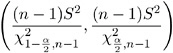
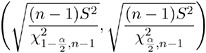
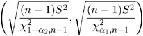
  In order to obtain a confidence interval for ƒ , the square root of each side is taken, leading to the following 100(1 ˆ’ ± )% confidence interval:

  

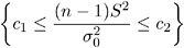
• The second method yields a confidence interval derived from the uniformly most powerful unbiased test of H : ƒ = ƒ (Lehmann 1986). This test has acceptance region

  

  where the critical values c ₁ and c ₂ satisfy

  

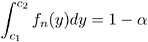
  and

  

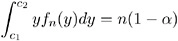
  where f _n ( y ) is the chi-squared distribution with n degrees of freedom. This acceptance region can be algebraically manipulated to arrive at

  

  where c ₁ and c ₂ solve the preceding two integrals. To find the area in each tail of the chi-square distribution to which these two critical values correspond , solve and for ± ₁ and ± ₂ ; the resulting ± ₁ and ± ₂ sum to ± . Hence, a 100(1 ˆ’ ± )% confidence interval for ƒ ² is given by

  

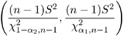
  In order to obtain a 100(1 ˆ’ ± )% confidence interval for ƒ , the square root is taken of both terms, yielding

  

Displayed Output

For each variable in the analysis, the TTEST procedure displays the following summary statistics for each group:

• the name of the dependent variable

• the levels of the classification variable

• N, the number of nonmissing values

• Lower CL Mean, the lower confidence bound for the mean

• the Mean or average

• Upper CL Mean, the upper confidence bound for the mean

• Lower CL Std Dev, the lower confidence bound for the standard deviation

• Std Dev, the standard deviation

• Upper CL Std Dev, the upper confidence bound for the standard deviation

• Std Err, the standard error of the mean

• the Minimum value, if the line size allows

• the Maximum value, if the line size allows

• upper and lower UMPU confidence bounds for the standard deviation, displayed if the CI=UMPU option is specified in the PROC TTEST statement

Next, the results of several t tests are given. For one-sample and paired observations t tests, the TTEST procedure displays

• t Value, the t statistic for testing the null hypothesis that the mean of the group is zero

• DF, the degrees of freedom

• Pr > t, the probability of a greater absolute value of t under the null hypothesis. This is the two-tailed significance probability.

To compute the one-tailed significance probability, first determine whether large values of t are significant or small values are. Let p denote the significance probability for the two-tailed test. If large values of t are significant, then the one-tailed probability is p/ 2 if t ‰ 0, and is 1 ˆ’ p/ 2 if t < 0. If small values of t are significant, then the one-tailed probability is 1 ˆ’ p/ 2 if t ‰ 0, and is p/ 2 if t < 0.

For two-sample t tests, the TTEST procedure displays all the items in the following list. You need to decide whether equal or unequal variances are appropriate for your data.

• Under the assumption of unequal variances, the TTEST procedure displays results using Satterthwaite's method. If the COCHRAN option is specified, the results for the Cochran and Cox approximation are also displayed.

  • t Value, an approximate t statistic for testing the null hypothesis that the means of the two groups are equal

  • DF, the approximate degrees of freedom

  • Pr > t, the probability of a greater absolute value of t under the null hypothesis. This is the two-tailed significance probability. The one-tailed probability is computed the same way as in a one-sample t test.

• Under the assumption of equal variances, the TTEST procedure displays results obtained by pooling the group variances.

  • t Value, the t statistic for testing the null hypothesis that the means of the two groups are equal

  • DF, the degrees of freedom

  • Pr > t, the probability of a greater absolute value of t under the null hypothesis. This is the two-tailed significance probability. The one-tailed probability is computed the same way as in a one-sample t test.

• PROC TTEST then gives the results of the test of equality of variances:

  • the F ² (folded) statistic (see the 'The Folded Form F Statistic' section on page 4784)

  • Num DF and Den DF, the numerator and denominator degrees of freedom in each group

  • Pr > F, the probability of a greater F ² value. This is the two-tailed significance probability.

ODS Table Names

PROC TTEST assigns a name to each table it creates. You can use these names to reference the table when using the Output Delivery System (ODS) to select tables and create output data sets. These names are listed in the following table. For more information on ODS, see Chapter 14, 'Using the Output Delivery System.'

Table 77.1: ODS Tables Produced in PROC TTEST

ODS Table Name	Description	Statement
Equality	Tests for equality of variance	CLASS statement
Statistics	Univariate summary statistics	by default
TTests	t -tests	by default