Examples
Example 75.1. Using Splines and Knots
This example illustrates some properties of splines. Splines are curves, which are usually required to be continuous and smooth. Splines are usually defined as piecewise polynomials of degree n with function values and first n ˆ’ 1 derivatives that agree at the points where they join. The abscissa values of the join points are called knots . The term 'spline' is also used for polynomials (splines with no knots) and piecewise polynomials with more than one discontinuous derivative. Splines with no knots are generally smoother than splines with knots, which are generally smoother than splines with multiple discontinuous derivatives. Splines with few knots are generally smoother than splines with many knots; however, increasing the number of knots usually increases the fit of the spline function to the data. Knots give the curve freedom to bend to more closely follow the data. Refer to Smith (1979) for an excellent introduction to splines.
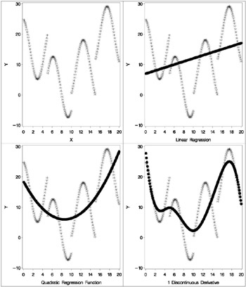
In this example, an artificial data set is created with a variable Y that is a discontinuous function of X .See the first plot in Output 75.1.7. Notice that the function has four unconnected parts , each of which is a curve. Notice too that there is an overall quadratic trend, that is, ignoring the shapes of the individual curves, at first the Y values tend to decrease as X increases, then Y values tend to increase.
| |
| |
The first PROC TRANSREG analysis fits a linear regression model. The predicted values of Y given X are output and plotted to form the linear regression line. The R 2 for the linear regression is 0.10061, and it can be seen from the second plot in Output 75.1.7 that the linear regression model is not appropriate for these data. The following statements create the data set and perform the first PROC TRANSREG analysis. These statements produce Output 75.1.1.
title 'An Illustration of Splines and Knots'; * Create in Y a discontinuous function of X. * * Store copies of X in V1-V7 for use in PROC GPLOT. * These variables are only necessary so that each * plot can have its own x-axis label while putting * four plots on a page.; data A; array V[7] V1-V7; X=-0.000001; do I=0 to 199; if mod(I,50)=0 then do; C=((X/2)-5)**2; if I=150 then C=C+5; Y=C; end; X=X+0.1; Y=Y-sin(X-C); do J=1 to 7; V[J]=X; end; output; end; run; * Each of the PROC TRANSREG steps fits a * different spline model to the data set created * previously. The TRANSREG steps build up a data set with * various regression functions. All of the functions * are then plotted with the final PROC GPLOT step. * * The OUTPUT statements add new predicted values * variables to the data set, while the ID statements * save all of the previously created variables that * are needed for the plots.; proc transreg data=A; model identity(Y) = identity(X); title2 'A Linear Regression Function'; output out=A pprefix=Linear; id V1-V7; run;
| |
An Illustration of Splines and Knots A Linear Regression Function The TRANSREG Procedure TRANSREG Univariate Algorithm Iteration History for Identity(Y) Iteration Average Maximum Criterion Number Change Change R-Square Change Note ------------------------------------------------------------------------- 1 0.00000 0.00000 0.10061 Converged Algorithm converged.
| |
The second PROC TRANSREG analysis finds a degree two spline transformation with no knots, which is a quadratic polynomial. The spline is a weighted sum of a single constant, a single straight line, and a single quadratic curve. The R 2 increases from 0.10061, which is the linear fit value from before, to 0.40720. It can be seen from the third plot in Output 75.1.7 that the quadratic regression function does not fit any of the individual curves well, but it does follow the overall trend in the data. Since the overall trend is quadratic, a degree three spline with no knots (not shown) increases R 2 by only a small amount. The following statements perform the quadratic analysis and produce Output 75.1.2.
proc transreg data=A; model identity(Y)=spline(X / degree=2); title2 'A Quadratic Polynomial Regression Function'; output out=A pprefix=Quad; id V1-V7 LinearY; run;
| |
An Illustration of Splines and Knots A Quadratic Polynomial Regression Function The TRANSREG Procedure TRANSREG MORALS Algorithm Iteration History for Identity(Y) Iteration Average Maximum Criterion Number Change Change R-Square Change Note ------------------------------------------------------------------------- 1 0.82127 2.77121 0.10061 2 0.00000 0.00000 0.40720 0.30659 Converged Algorithm converged.
| |
The next step uses the default degree of three, for a piecewise cubic polynomial, and requests knots at the known break points, X =5, 10, and 15. This requests a spline that is continuous, has continuous first and second derivatives, and has a third derivative that is discontinuous at 5, 10, and 15. The spline is a weighted sum of a single constant, a single straight line, a single quadratic curve, a cubic curve for the portion of X less than 5, a different cubic curve for the portion of X between 5 and 10, a different cubic curve for the portion of X between 10 and 15, and another cubic curve for the portion of X greater than 15. The new R 2 is 0.61730, and it can be seen from the fourth plot (in Output 75.1.7) that the spline is less smooth than the quadratic polynomial and it follows the data more closely than the quadratic polynomial. The following statements perform this analysis and produce Output 75.1.3:
proc transreg data=A; model identity(Y) = spline(X / knots=5 10 15); title2 'A Cubic Spline Regression Function'; title3 'The Third Derivative is Discontinuous at X=5, 10, 15'; output out=A pprefix=Cub1; id V1-V7 LinearY QuadY; run;
| |
An Illustration of Splines and Knots A Cubic Spline Regression Function The Third Derivative is Discontinuous at X=5, 10, 15 The TRANSREG Procedure TRANSREG MORALS Algorithm Iteration History for Identity(Y) Iteration Average Maximum Criterion Number Change Change R-Square Change Note ------------------------------------------------------------------------- 1 0.85367 3.88449 0.10061 2 0.00000 0.00000 0.61730 0.51670 Converged Algorithm converged.
| |
The same model could be fit with a DATA step and PROC REG, as follows. (The output from the following code is not displayed.)
data B; /* A is the data set used for transreg */ set a(keep=X Y); X1=X; /* X */ X2=X**2; /* X squared */ X3=X**3; /* X cubed */ X4=(X> 5)*((X-5)**3); /* change in X**3 after 5 */ X5=(X>10)*((X-10)**3); /* change in X**3 after 10 */ X6=(X>15)*((X-15)**3); /* change in X**3 after 15 */ run; proc reg; model Y=X1-X6; run;
In the next step each knot is repeated three times, so the first, second, and third derivatives are discontinuous at X =5, 10, and 15, but the spline is required to be continuous at the knots. The spline is a weighted sum of the following.
-
a single constant
-
a line for the portion of X less than 5
-
a quadratic curve for the portion of X less than 5
-
a cubic curve for the portion of X less than 5
-
a different line for the portion of X between 5 and 10
-
a different quadratic curve for the portion of X between 5 and 10
-
a different cubic curve for the portion of X between 5 and 10
-
a different line for the portion of X between 10 and 15
-
a different quadratic curve for the portion of X between 10 and 15
-
a different cubic curve for the portion of X between 10 and 15
-
another line for the portion of X greater than 15
-
another quadratic curve for the portion of X greater than 15
-
and another cubic curve for the portion of X greater than 15
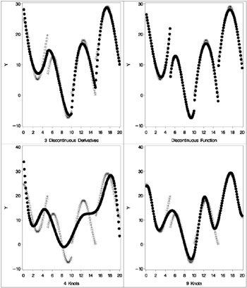
The spline is continuous since there is not a separate constant in the formula for the spline for each knot. Now the R 2 is 0.95542, and the spline closely follows the data, except at the knots. The following statements perform this analysis and produce Output 75.1.4:
proc transreg data=A; model identity(y) = spline(x / knots=5 5 5 10 10 10 15 15 15); title3 'First - Third Derivatives Discontinuous at X=5, 10, 15'; output out=A pprefix=Cub3; id V1-V7 LinearY QuadY Cub1Y; run;
| |
An Illustration of Splines and Knots A Cubic Spline Regression Function First - Third Derivatives Discontinuous at X=5, 10, 15 The TRANSREG Procedure TRANSREG MORALS Algorithm Iteration History for Identity(Y) Iteration Average Maximum Criterion Number Change Change R-Square Change Note ------------------------------------------------------------------------- 1 0.92492 3.50038 0.10061 2 0.00000 0.00000 0.95542 0.85481 Converged Algorithm converged.
| |
The same model could be fit with a DATA step and PROC REG, as follows. (The output from the following code is not displayed.)
data B; set a(keep=X Y); X1=X; /* X */ X2=X**2; /* X squared */ X3=X**3; /* X cubed */ X4=(X>5) * (X- 5); /* change in X after 5 */ X5=(X>10) * (X-10); /* change in X after 10 */ X6=(X>15) * (X-15); /* change in X after 15 */ X7=(X>5) * ((X-5)**2); /* change in X**2 after 5 */ X8=(X>10) * ((X-10)**2); /* change in X**2 after 10 */ X9=(X>15) * ((X-15)**2); /* change in X**2 after 15 */ X10=(X>5) * ((X-5)**3); /* change in X**3 after 5 */ X11=(X>10) * ((X-10)**3); /* change in X**3 after 10 */ X12=(X>15) * ((X-15)**3); /* change in X**3 after 15 */ run; proc reg; model Y=X1-X12; run;
When the knots are repeated four times in the next step, the spline function is discontinuous at the knots and follows the data even more closely, with an R 2 of 0.99254. In this step, each separate curve is approximated by a cubic polynomial (with no knots within the separate polynomials). The following statements perform this analysis and produce Output 75.1.5:
proc transreg data=A; model identity(Y) = spline(X / knots=5 5 5 5 10 10 10 10 15 15 15 15); title3 'Discontinuous Function and Derivatives'; output out=A pprefix=Cub4; id V1-V7 LinearY QuadY Cub1Y Cub3Y; run;
| |
An Illustration of Splines and Knots A Cubic Spline Regression Function Discontinuous Function and Derivatives The TRANSREG Procedure TRANSREG MORALS Algorithm Iteration History for Identity(Y) Iteration Average Maximum Criterion Number Change Change R-Square Change Note ------------------------------------------------------------------------- 1 0.90271 3.29184 0.10061 2 0.00000 0.00000 0.99254 0.89193 Converged Algorithm converged.
| |
To solve this problem with a DATA step and PROC REG, you would need to create all of the variables in the preceding DATA step (the B data set for the piecewise polynomial with discontinuous third derivatives), plus the following three variables.
X13=(X > 5); /* intercept change after 5 */ X14=(X > 10); /* intercept change after 10 */ X15=(X > 15); /* intercept change after 15 */
The last two steps use the NKNOTS= t-option to specify the number of knots but not their location. NKNOTS=4 places knots at the quintiles while NKNOTS=9 places knots at the deciles. The spline and its first two derivatives are continuous. The R 2 values are 0.74450 and 0.95256. Even though the knots are placed in the wrong places, the spline can closely follow the data with NKNOTS=9. The following statements produce Output 75.1.6.
proc transreg data=A; model identity(Y) = spline(X / nknots=4); title3 'Four Knots'; output out=A pprefix=Cub4k; id V1-V7 LinearY QuadY Cub1Y Cub3Y Cub4Y; run; proc transreg data=A; model identity(Y) = spline(X / nknots=9); title3 'Nine Knots'; output out=A pprefix=Cub9k; id V1-V7 LinearY QuadY Cub1Y Cub3Y Cub4Y Cub4kY; run;
| |
An Illustration of Splines and Knots A Cubic Spline Regression Function Four Knots The TRANSREG Procedure TRANSREG MORALS Algorithm Iteration History for Identity(Y) Iteration Average Maximum Criterion Number Change Change R-Square Change Note ------------------------------------------------------------------------- 1 0.90305 4.46027 0.10061 2 0.00000 0.00000 0.74450 0.64389 Converged Algorithm converged. An Illustration of Splines and Knots A Cubic Spline Regression Function Nine Knots The TRANSREG Procedure TRANSREG MORALS Algorithm Iteration History for Identity(Y) Iteration Average Maximum Criterion Number Change Change R-Square Change Note ------------------------------------------------------------------------- 1 0.94832 3.03488 0.10061 2 0.00000 0.00000 0.95256 0.85196 Converged Algorithm converged.
| |
The following statements produce plots that show the data and fit at each step of the analysis. These statements produce Output 75.1.7.
goptions goutmode=replace nodisplay; %let opts = haxis=axis2 vaxis=axis1 frame cframe=ligr; * Depending on your goptions, these plot options may work better: * %let opts = haxis=axis2 vaxis=axis1 frame; proc gplot data=A; title; axis1 minor=none label=(angle=90 rotate=0); axis2 minor=none; plot Y*X=1 / &opts name='tregdis1'; plot Y*V1=1 linearY*X=2 /overlay &opts name='tregdis2'; plot Y*V2=1 quadY *X=2 /overlay &opts name='tregdis3'; plot Y*V3=1 cub1Y *X=2 /overlay &opts name='tregdis4'; plot Y*V4=1 cub3Y *X=2 /overlay &opts name='tregdis5'; plot Y*V5=1 cub4Y *X=2 /overlay &opts name='tregdis6'; plot Y*V6=1 cub4kY *X=2 /overlay &opts name='tregdis7'; plot Y*V7=1 cub9kY *X=2 /overlay &opts name='tregdis8'; symbol1 color=blue v=star i=none; symbol2 color=yellow v=dot i=none; label V1 = 'Linear Regression' V2 = 'Quadratic Regression Function' V3 = '1 Discontinuous Derivative' V4 = '3 Discontinuous Derivatives' V5 = 'Discontinuous Function' V6 = '4 Knots' V7 = '9 Knots' Y = 'Y' LinearY = 'Y' QuadY = 'Y' Cub1Y = 'Y' Cub3Y = 'Y' Cub4Y = 'Y' Cub4kY = 'Y' Cub9kY = 'Y'; run; quit; goptions display; proc greplay nofs tc=sashelp.templt template=l2r2; igout gseg; treplay 1:tregdis1 2:tregdis3 3:tregdis2 4:tregdis4; treplay 1:tregdis5 2:tregdis7 3:tregdis6 4:tregdis8; run; quit;
| |
| |
These next steps show how to find optimal spline transformations of variables in one data set and apply the same transformations to variables in another data set. These steps produce two artificial data sets, in which the variable Y is a linear function of nonlinear transformations of the variables X , W ,and Z .
title2 'Scoring Spline Variables'; data x; do i = 1 to 5000; w = normal(7); x = normal(7); z = normal(7); y = w * w + log(5 + x) + sin(z) + normal(7); output; end; run; data z; do i = 1 to 5000; w = normal(1); x = normal(1); z = normal(1); y = w * w + log(5 + x) + sin(z) + normal(1); output; end; run;
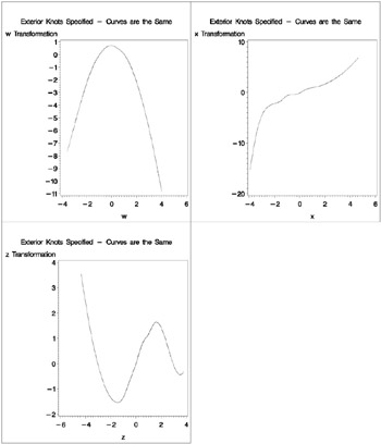
First, you run PROC TRANSREG asking for spline transformations of the three independent variables. You must use the EXKNOTS= t-option , because you need to use the same knots, both interior and exterior, with both data sets. By default the exterior knots will be different if the minima and maxima are different in the two data sets, so you will get the wrong results if you do not specify the EXKNOTS= t-option with values less than the minima and greater than the maxima of the two Y variables.
ods output splinecoef=c; proc transreg data=x dum det ss2; model ide(y) = spl(wxz/knots=-1.5 to 1.5 by 0.5 exknots=-5 5); output out=d; run;
The nonprinting 'SplineCoef' table is output to a SAS data set. This data set contains the coefficients used to get the spline transformations and can be used to transform variables in other data sets. These coefficients are also in the details table. However, in the 'SplineCoef' table they are in a form directly suitable for use with PROC SCORE.
This next step reads a different input data set and generates an output data set with the B-spline basis for each of the variables. Note that the same interior and exterior knots are used in both the previous and the next steps.
proc transreg data=z design; model bspl(wxz/knots= 1.5 to 1.5 by 0.5 exknots= 5 5); output out=b; run;
These next three steps score the B-spline bases created in the previous step using the coefficients generated in the first PROC TRANSREG step. PROC SCORE is run once for each SPLINE variable.
proc score data=b score=c out=o1(rename=(spline=bw w=nw)); var w:; run; proc score data=b score=c out=o2(rename=(spline=bx x=nx)); var x:; run; proc score data=b score=c out=o3(rename=(spline=bz z=nz)); var z:; run;
The next steps merge the three transformations with the original data and plot the results. The plots in Output 75.1.8 show that in fact the two transformations for each variable, original and scored, are the same function. Furthermore, PROC TRANSREG found the functional forms that were used to generate the data: quadratic for W , log for X , and sine for Z .
| |
| |
goptions goutmode=replace nodisplay; data all; merge d(keep=w x z tw tx tz) o1(keep=nw bw) o2(keep=nx bx) o3(keep=nz bz); run; proc gplot data=all; title3 'Exterior Knots Specified - Curves are the Same'; symbol1 color=blue v=none i=smooths; symbol2 color=red v=none i=smooths; plot tw * w = 1 bw * nw = 2 / overlay name='tregspl1'; plot tx * x = 1 bx * nx = 2 / overlay name='tregspl2'; plot tz * z = 1 bz * nz = 2 / overlay name='tregspl3'; run; quit; goptions display; proc greplay nofs tc=sashelp.templt template=l2r2; igout gseg; treplay 1:tregspl1 2:tregspl3 3:tregspl2; run; quit;
Example 75.2. Nonmetric Conjoint Analysis of Tire Data
This example uses PROC TRANSREG to perform a nonmetric conjoint analysis of tire preference data. Conjoint analysis decomposes rank ordered evaluation judgments of products or services into components based on qualitative product attributes.
For each level of each attribute of interest, a numerical 'part-worth utility' value is computed. The sum of the part-worth utilities for each product is an estimate of the utility for that product. The goal is to compute part-worth utilities such that the product utilities are as similar as possible to the original rank ordering. (This example is a greatly simplified introductory example.)
The stimuli for the experiment are 18 hypothetical tires. The stimuli represent different brands (Goodstone, Pirogi, Machismo), [*] prices ($69.99, $74.99, $79.99), expected tread life (50,000, 60,000, 70,000), and road hazard insurance plans (Yes, No). There are 3 — 3 — 3 — 2 = 54 possible combinations. From these, 18 combinations are selected that form an efficient experimental design for a main effects model. The combinations are then ranked from 1 (most preferred) to 18 (least preferred). In this simple example, there is one set of rankings. A real conjoint study would have many more.
First, the FORMAT procedure is used to specify the meanings of the factor levels, which are entered as numbers in the DATA step along with the ranks. PROC TRANSREG is used to perform the conjoint analysis. A maximum of 50 iterations is requested . The specification Monotone(Rank / Reflect) in the MODEL statement requests that the dependent variable Rank should be monotonically transformed and reflected so that positive utilities mean high preference. The variables Brand , Price , Life ,and Hazard are designated as CLASS variables, and the part-worth utilities are constrained by ZERO=SUM to sum to zero within each factor. The UTILITIES a-option displays the conjoint analysis results.
The Importance column of the Utilities Table shows that price is the most important attribute in determining preference (57%), followed by expected tread life (18%), brand (15%), and road hazard insurance (10%). Looking at the Utilities Table for the maximum part-worth utility within each attribute, you see from the results that the most preferred combination is Pirogi brand tires, at $69.99, with a 70,000 mile expected tread life, and road hazard insurance. This product is not actually in the data set. The sum of the part-worth utilities for this combination is
The following statements produce Output 75.2.1:
title 'Nonmetric Conjoint Analysis of Ranks'; proc format; value BrandF 1 = 'Goodstone' 2 = 'Pirogi ' 3 = 'Machismo '; value PriceF 1 = '.99' 2 = '.99' 3 = '.99'; value LifeF 1 = '50,000' 2 = '60,000' 3 = '70,000'; value HazardF 1 = 'Yes' 2 = 'No '; run; data Tires; input Brand Price Life Hazard Rank; format Brand BrandF9. Price PriceF9. Life LifeF6. Hazard HazardF3.; datalines; 1 1 2 1 3 1 1 3 2 2 1 2 1 2 14 1 2 2 2 10 1 3 1 1 17 1 3 3 1 12 2 1 1 2 7 2 1 3 2 1 2 2 1 1 8 2 2 3 1 5 2 3 2 1 13 2 3 2 2 16 3 1 1 1 6 3 1 2 1 4 3 2 2 2 15 3 2 3 1 9 3 3 1 2 18 3 3 3 2 11 ; proc transreg maxiter=50 utilities short; ods select ConvergenceStatus FitStatistics Utilities; model monotone(Rank / reflect) = class(Brand Price Life Hazard / zero=sum); output ireplace predicted; run; proc print label; var Rank TRank PRank Brand Price Life Hazard; label PRank = 'Predicted Ranks'; run;
| |
Nonmetric Conjoint Analysis of Ranks The TRANSREG Procedure Monotone(Rank) Algorithm converged. The TRANSREG Procedure Hypothesis Tests for Monotone(Rank) Root MSE 0.49759 R-Square 0.9949 Dependent Mean 9.50000 Adj R-Sq 0.9913 Coeff Var 5.23783 Utilities Table Based on the Usual Degrees of Freedom Importance Standard (% Utility Label Utility Error Range) Variable Intercept 9.5000 0.11728 Intercept Brand Goodstone 1.1718 0.16586 15.463 Class.BrandGoodstone Brand Pirogi 1.8980 0.16586 Class.BrandPirogi Brand Machismo 0.7262 0.16586 Class.BrandMachismo Price .99 5.8732 0.16586 56.517 Class.Price_69_99 Price .99 0.5261 0.16586 Class.Price_74_99 Price .99 5.3471 0.16586 Class.Price_79_99 Life 50,000 1.2350 0.16586 18.361 Class.Life50_000 Life 60,000 1.1751 0.16586 Class.Life60_000 Life 70,000 2.4101 0.16586 Class.Life70_000 Hazard Yes 0.9588 0.11728 9.659 Class.HazardYes Hazard No 0.9588 0.11728 Class.HazardNo The standard errors are not adjusted for the fact that the dependent variable was transformed and so are generally liberal (too small). Nonmetric Conjoint Analysis of Ranks Rank Predicted Obs Rank Transformation Ranks Brand Price Life Hazard 1 3 14.4462 13.9851 Goodstone .99 60,000 Yes 2 2 15.6844 15.6527 Goodstone .99 70,000 No 3 14 5.7229 5.6083 Goodstone .99 50,000 No 4 10 5.7229 5.6682 Goodstone .99 60,000 No 5 17 2.6699 2.7049 Goodstone .99 50,000 Yes 6 12 5.7229 6.3500 Goodstone .99 70,000 Yes 7 7 14.4462 15.0774 Pirogi .99 50,000 No 8 1 18.7699 18.7225 Pirogi .99 70,000 No 9 8 11.1143 10.5957 Pirogi .99 50,000 Yes 10 5 14.4462 14.2408 Pirogi .99 70,000 Yes 11 13 5.7229 5.8346 Pirogi .99 60,000 Yes 12 16 3.8884 3.9170 Pirogi .99 60,000 No 13 6 14.4462 14.3708 Machismo .99 50,000 Yes 14 4 14.4462 14.4307 Machismo .99 60,000 Yes 15 15 5.7229 6.1139 Machismo .99 60,000 No 16 9 11.1143 11.6166 Machismo .99 70,000 Yes 17 18 1.1905 1.2330 Machismo .99 50,000 No 18 11 5.7229 4.8780 Machismo .99 70,000 No
| |
Example 75.3. Metric Conjoint Analysis of Tire Data
This example, which is more detailed than the previous one, uses PROC TRANSREG to perform a metric conjoint analysis of tire preference data. Conjoint analysis can be used to decompose preference ratings of products or services into components based on qualitative product attributes. For each level of each attribute of interest, a numerical 'part-worth utility' value is computed. The sum of the part-worth utilities for each product is an estimate of the utility for that product. The goal is to compute part-worth utilities such that the product utilities are as similar as possible to the original ratings. Metric conjoint analysis, as shown in this example, fits an ordinary linear model directly to data assumed to be measured on an interval scale. Nonmetric conjoint analysis, as shown in Example 75.2, finds an optimal monotonic transformation of original data before fitting an ordinary linear model to the transformed data.
This example has three parts. In the first part, an experimental design is created. In the second part, a DATA step creates descriptions of the stimuli for the experiment. The third part of the example performs the conjoint analyses.
The stimuli for the experiment are 18 hypothetical tires. The stimuli represent different brands (Goodstone, Pirogi, Machismo), [*] prices ($69.99, $74.99, $79.99), expected tread life (50,000, 60,000, 70,000), and road hazard insurance plans (Yes, No).
For a conjoint study such as this, you need to create an experimental design with 3 three-level factors, 1 two-level factor, and 18 combinations or runs . The easiest way to get this design is with the %MktEx autocall macro. The %MktEx macro requires you to specify the number of levels of each of the four factors, followed by N=18, the number of runs. Specifying a random number seed, while not strictly necessary, helps ensure that the design is reproducible. The %MktLab macro assigns the actual factor names instead of the default names X1, X2, and so on, and it assigns formats to the factor levels. The %MktEval macro helps you evaluate the design. It shows how correlated or independent the factors are, how often each factor level appears in the design, how often each pair occurs for every factor pair, and how often each product profile or run occurs in the design. See Kuhfeld (2003) for more information on these tools and their use in conjoint and choice modeling.
title 'Tire Study, Experimental Design'; proc format; value BrandF 1 = 'Goodstone' 2 = 'Pirogi ' 3 = 'Machismo '; value PriceF 1 = '.99' 2 = '.99' 3 = '.99'; value LifeF 1 = '50,000' 2 = '60,000' 3 = '70,000'; value HazardF 1 = 'Yes' 2 = 'No ';(persist run; %mktex(3 3 3 2, n=18, seed=448) %mktlab(vars=Brand Price Life Hazard, out=sasuser.TireDesign, statements=format Brand BrandF9. Price PriceF9. Life LifeF6. Hazard HazardF3.) %mkteval; proc print data=sasuser.TireDesign; run;
The %MktEx macro output displayed in Output 75.3.1 shows you that the design is 100% efficient, which means it is orthogonal and balanced. The %MktEval macro output displayed in Output 75.3.2 shows you that all of the factors are uncorrelated or orthogonal, the design is balanced (each level occurs once), and every pair of factor levels occurs equally often (again showing that the design is orthogonal). The n -way frequencies show that each product profile occurs once (there are no duplicates). The design is shown in Output 75.3.3. The design is automatically randomized (the profiles were sorted into a random order and the original levels are randomly reassigned). Orthogonality, balance, randomization, and other design concepts are discussed in detail in Kuhfeld (2003).
| |
Tire Study, Experimental Design Algorithm Search History Current Best Design Row,Col D-Efficiency D-Efficiency Notes ---------------------------------------------------------- 1 Start 100.0000 100.0000 Tab 1 End 100.0000 Tire Study, Experimental Design The OPTEX Procedure Class Level Information Class Levels -Values- x1 3 1 2 3 x2 3 1 2 3 x3 3 1 2 3 x4 2 1 2 Tire Study, Experimental Design The OPTEX Procedure Average Prediction Design Standard Number D-Efficiency A-Efficiency G-Efficiency Error ------------------------------------------------------------------------ 1 100.0000 100.0000 100.0000 0.6667
| |
| |
Canonical Correlations Between the Factors There are 0 Canonical Correlations Greater Than 0.316 Brand Price Life Hazard Brand 1 0 0 0 Price 0 1 0 0 Life 0 0 1 0 Hazard 0 0 0 1 Summary of Frequencies There are 0 Canonical Correlations Greater Than 0.316 Frequencies Brand 6 6 6 Price 6 6 6 Life 6 6 6 Hazard 9 9 Brand Price 2 2 2 2 2 2 2 2 2 Brand Life 2 2 2 2 2 2 2 2 2 Brand Hazard 3 3 3 3 3 3 Price Life 2 2 2 2 2 2 2 2 2 Price Hazard 3 3 3 3 3 3 Life Hazard 3 3 3 3 3 3 N-Way 1 1 1 1 1 1 1 1 1 1 1 1 1 1 1 1 1 1
| |
| |
Obs Brand Price Life Hazard 1 Pirogi .99 50,000 No 2 Machismo .99 70,000 No 3 Machismo .99 50,000 Yes 4 Machismo .99 50,000 No 5 Goodstone .99 70,000 Yes 6 Pirogi .99 70,000 Yes 7 Goodstone .99 50,000 Yes 8 Machismo .99 60,000 Yes 9 Pirogi .99 60,000 Yes 10 Pirogi .99 60,000 No 11 Goodstone .99 60,000 No 12 Goodstone .99 50,000 No 13 Pirogi .99 50,000 Yes 14 Goodstone .99 70,000 No 15 Machismo .99 60,000 No 16 Machismo .99 70,000 Yes 17 Pirogi .99 70,000 No 18 Goodstone .99 60,000 Yes
| |
Next, the questionnaires are printed, and subjects are given the questionnaires and are asked to rate the tires.
The following statements produce Output 75.3.4. This output is abbreviated; the statements produce stimuli for all combinations.
data _null_; title; set sasuser.TireDesign; file print; if mod(_n_,4) eq 1 then do; put _page_; put +55 'Subject ________'; end; length hazardstring $ 7.; if put(hazard, hazardf3.) = 'Yes' then hazardstring = 'with'; else hazardstring = 'without'; s = 3 + (_n_ >= 10); put // _n_ +(-1) ') For your next tire purchase ' 'how likely are you to buy this product?' // +s Brand 'brand tires at ' Price +( 1) ',' / +s 'with a ' Life 'tread life guarantee, ' / +s 'and ' hazardstring 'road hazard insurance.' // +s 'Definitely Would Definitely Would' / +s 'Not Purchase Purchase' // +s '1 2 3 4 5 6 7 8 9 '; run; | |
Subject ________ 1) For your next tire purchase, how likely are you to buy this product? Pirogi brand tires at .99, with a 50,000 tread life guarantee, and without road hazard insurance. Definitely Would Definitely Would Not Purchase Purchase 1 2 3 4 5 6 7 8 9 2) For your next tire purchase, how likely are you to buy this product? Machismo brand tires at .99, with a 70,000 tread life guarantee, and without road hazard insurance. Definitely Would Definitely Would Not Purchase Purchase 1 2 3 4 5 6 7 8 9 3) For your next tire purchase, how likely are you to buy this product? Machismo brand tires at .99, with a 50,000 tread life guarantee, and with road hazard insurance. Definitely Would Definitely Would Not Purchase Purchase 1 2 3 4 5 6 7 8 9 4) For your next tire purchase, how likely are you to buy this product? Machismo brand tires at .99, with a 50,000 tread life guarantee, and without road hazard insurance. Definitely Would Definitely Would Not Purchase Purchase 1 2 3 4 5 6 7 8 9
| |
The third part of the example performs the conjoint analyses. The DATA step reads the data. Only the ratings are entered, one row per subject. Real conjoint studies have many more subjects than five. The TRANSPOSE procedure transposes this (5 — 18) data set into an (18 — 5) data set that can be merged with the factor level data set sasuser.TireDesign . The next DATA step does the merge. The PRINT procedure displays the input data set.
PROC TRANSREG fits the five individual conjoint models, one for each subject. The UTILITIES a-option displays the conjoint analysis results. The SHORT a-option suppresses the iteration histories, OUTTEST= Utils creates an output data set with all of the conjoint results, and the SEPARATORS= option requests that the labels constructed for each category contain two blanks between the variable name and the level value. The ODS select statement is used to limit the displayed output. The MODEL statement specifies IDENTITY for the ratings, which specifies a metric conjoint analysis -the ratings are not transformed. The variables Brand , Price , Life ,and Hazard are designated as CLASS variables, and the part-worth utilities are constrained to sum to zero within each factor.
The following statements produce Output 75.3.5:
title 'Tire Study, Data Entry, Preprocessing'; data Results; input (c1-c18) (1.); datalines; 233279766526376493 124467885349168274 262189456534275794 184396375364187754 133379775526267493 ; *---Create an Object by Subject Data Matrix---; proc transpose data=Results out=Results(drop=_name_) prefix=Subj; run; *---Merge the Factor Levels With the Data Matrix---; data Both; merge sasuser.TireDesign Results; run; *---Print Input Data Set---; proc print; title2 'Data Set for Conjoint Analysis'; run; *---Fit Each Subject Individually---; proc transreg data=Both utilities short outtest=Utils separators=' '; ods select TestsNote FitStatistics Utilities; title2 'Individual Conjoint Analyses'; model identity(Subj1-Subj5) = class(Brand Price Life Hazard / zero=sum); run;
| |
Tire Study, Data Entry, Preprocessing Data Set for Conjoint Analysis Obs Brand Price Life Hazard Subj1 Subj2 Subj3 Subj4 Subj5 1 Pirogi .99 50,000 No 2 1 2 1 1 2 Machismo .99 70,000 No 3 2 6 8 3 3 Machismo .99 50,000 Yes 3 4 2 4 3 4 Machismo .99 50,000 No 2 4 1 3 3 5 Goodstone .99 70,000 Yes 7 6 8 9 7 6 Pirogi .99 70,000 Yes 9 7 9 6 9 7 Goodstone .99 50,000 Yes 7 8 4 3 7 8 Machismo .99 60,000 Yes 6 8 5 7 7 9 Pirogi .99 60,000 Yes 6 5 6 5 5 10 Pirogi .99 60,000 No 5 3 5 3 5 11 Goodstone .99 60,000 No 2 4 3 6 2 12 Goodstone .99 50,000 No 6 9 4 4 6 13 Pirogi .99 50,000 Yes 3 1 2 1 2 14 Goodstone .99 70,000 No 7 6 7 8 6 15 Machismo .99 60,000 No 6 8 5 7 7 16 Machismo .99 70,000 Yes 4 2 7 7 4 17 Pirogi .99 70,000 No 9 7 9 5 9 18 Goodstone .99 60,000 Yes 3 4 4 4 3 Tire Study, Data Entry, Preprocessing Individual Conjoint Analyses The TRANSREG Procedure The TRANSREG Procedure Hypothesis Tests for Identity(Subj1) Root MSE 0.44721 R-Square 0.9783 Dependent Mean 5.00000 Adj R-Sq 0.9630 Coeff Var 8.94427 Utilities Table Based on the Usual Degrees of Freedom Importance Standard (% Utility Label Utility Error Range) Variable Intercept 5.0000 0.10541 Intercept Brand Goodstone 0.3333 0.14907 17.857 Class.BrandGoodstone Brand Pirogi 0.6667 0.14907 Class.BrandPirogi Brand Machismo 1.0000 0.14907 Class.BrandMachismo Price .99 2.1667 0.14907 46.429 Class.Price_69_99 Price .99 0.0000 0.14907 Class.Price_74_99 Price .99 2.1667 0.14907 Class.Price_79_99 Life 50,000 1.1667 0.14907 28.571 Class.Life50_000 Life 60,000 0.3333 0.14907 Class.Life60_000 Life 70,000 1.5000 0.14907 Class.Life70_000 Hazard Yes 0.3333 0.10541 7.143 Class.HazardYes Hazard No 0.3333 0.10541 Class.HazardNo Tire Study, Data Entry, Preprocessing Individual Conjoint Analyses The TRANSREG Procedure The TRANSREG Procedure Hypothesis Tests for Identity(Subj2) Root MSE 0.50553 R-Square 0.9770 Dependent Mean 4.94444 Adj R-Sq 0.9608 Coeff Var 10.22410 Utilities Table Based on the Usual Degrees of Freedom Importance Standard (% Utility Label Utility Error Range) Variable Intercept 4.9444 0.11915 Intercept Brand Goodstone 1.2222 0.16851 25.161 Class.BrandGoodstone Brand Pirogi 0.9444 0.16851 Class.BrandPirogi Brand Machismo 0.2778 0.16851 Class.BrandMachismo Price .99 2.8889 0.16851 63.871 Class.Price_69_99 Price .99 0.2778 0.16851 Class.Price_74_99 Price .99 2.6111 0.16851 Class.Price_79_99 Life 50,000 0.4444 0.16851 9.677 Class.Life50_000 Life 60,000 0.3889 0.16851 Class.Life60_000 Life 70,000 0.0556 0.16851 Class.Life70_000 Hazard Yes 0.0556 0.11915 1.290 Class.HazardYes Hazard No 0.0556 0.11915 Class.HazardNo Tire Study, Data Entry, Preprocessing Individual Conjoint Analyses The TRANSREG Procedure The TRANSREG Procedure Hypothesis Tests for Identity(Subj2) Root MSE 0.50553 R-Square 0.9770 Dependent Mean 4.94444 Adj R-Sq 0.9608 Coeff Var 10.22410 Utilities Table Based on the Usual Degrees of Freedom Importance Standard (% Utility Label Utility Error Range) Variable Intercept 4.9444 0.11915 Intercept Brand Goodstone 1.2222 0.16851 25.161 Class.BrandGoodstone Brand Pirogi 0.9444 0.16851 Class.BrandPirogi Brand Machismo 0.2778 0.16851 Class.BrandMachismo Price .99 2.8889 0.16851 63.871 Class.Price_69_99 Price .99 0.2778 0.16851 Class.Price_74_99 Price .99 2.6111 0.16851 Class.Price_79_99 Life 50,000 0.4444 0.16851 9.677 Class.Life50_000 Life 60,000 0.3889 0.16851 Class.Life60_000 Life 70,000 0.0556 0.16851 Class.Life70_000 Hazard Yes 0.0556 0.11915 1.290 Class.HazardYes Hazard No 0.0556 0.11915 Class.HazardNo Tire Study, Data Entry, Preprocessing Individual Conjoint Analyses The TRANSREG Procedure The TRANSREG Procedure Hypothesis Tests for Identity(Subj4) Root MSE 0.92496 R-Square 0.9099 Dependent Mean 5.05556 Adj R-Sq 0.8468 Coeff Var 18.29596 Utilities Table Based on the Usual Degrees of Freedom Importance Standard (% Utility Label Utility Error Range) Variable Intercept 5.0556 0.21802 Intercept Brand Goodstone 0.6111 0.30832 31.469 Class.BrandGoodstone Brand Pirogi 1.5556 0.30832 Class.BrandPirogi Brand Machismo 0.9444 0.30832 Class.BrandMachismo Price .99 0.2778 0.30832 10.490 Class.Price_69_99 Price .99 0.2778 0.30832 Class.Price_74_99 Price .99 0.5556 0.30832 Class.Price_79_99 Life 50,000 2.3889 0.30832 56.643 Class.Life50_000 Life 60,000 0.2778 0.30832 Class.Life60_000 Life 70,000 2.1111 0.30832 Class.Life70_000 Hazard Yes 0.0556 0.21802 1.399 Class.HazardYes Hazard No 0.0556 0.21802 Class.HazardNo Tire Study, Data Entry, Preprocessing Individual Conjoint Analyses The TRANSREG Procedure The TRANSREG Procedure Hypothesis Tests for Identity(Subj5) Root MSE 0.34960 R-Square 0.9879 Dependent Mean 4.94444 Adj R-Sq 0.9794 Coeff Var 7.07062 Utilities Table Based on the Usual Degrees of Freedom Importance Standard (% Utility Label Utility Error Range) Variable Intercept 4.9444 0.08240 Intercept Brand Goodstone 0.2222 0.11653 7.500 Class.BrandGoodstone Brand Pirogi 0.2222 0.11653 Class.BrandPirogi Brand Machismo 0.4444 0.11653 Class.BrandMachismo Price .99 2.5556 0.11653 56.250 Class.Price_69_99 Price .99 0.1111 0.11653 Class.Price_74_99 Price .99 2.4444 0.11653 Class.Price_79_99 Life 50,000 1.2778 0.11653 30.000 Class.Life50_000 Life 60,000 0.1111 0.11653 Class.Life60_000 Life 70,000 1.3889 0.11653 Class.Life70_000 Hazard Yes 0.2778 0.08240 6.250 Class.HazardYes Hazard No 0.2778 0.08240 Class.HazardNo
| |
The output contains two tables per subject, one with overall fit statistics and one with the conjoint analysis results.
These following statements summarize the results. Three tables are displayed: all of the importance values, the average importance, and the part-worth utilities. The first DATA step selects the importance information from the Utils data set. The final assignment statement stores just the variable name from the label relying on the fact that the separator is two blanks. PROC TRANSPOSE creates the data set of importances, one row per subject, and PROC PRINT displays the results. The MEANS procedure displays the average importance of each attribute across the subjects. The next DATA step selects the part-worth utilities information from the Utils data set. PROC TRANSPOSE creates the data set of utilities, one row per subject, and PROC PRINT displays the results.
*---Gather the Importance Values---; data Importance; set Utils(keep=_depvar_ Importance Label); if n(Importance); label = substr(label, 1, index(label, ' ')); run; proc transpose out=Importance2(drop=_:); by _depvar_; id Label; run; proc print; title2 'Importance Values'; run; proc means; title2 'Average Importance'; run; *---Gather the Part-Worth Utilites--- ; data Utilities; set Utils(keep=_depvar_ Coefficient Label); if n(Coefficient); run; proc transpose out=Utilities2(drop=_:); by _depvar_; id Label; idlabel Label; run; proc print label; title2 'Utilities'; run;
| |
Tire Study, Data Entry, Preprocessing Importance Values Obs Brand Price Life Hazard 1 17.8571 46.4286 28.5714 7.14286 2 25.1613 63.8710 9.6774 1.29032 3 13.1250 22.5000 58.1250 6.25000 4 31.4685 10.4895 56.6434 1.39860 5 7.5000 56.2500 30.0000 6.25000 Tire Study, Data Entry, Preprocessing Average Importance The MEANS Procedure Variable N Mean Std Dev Minimum Maximum ------------------------------------------------------------------------------ Brand 5 19.0223929 9.5065111 7.5000000 31.4685315 Price 5 39.9078099 22.6510962 10.4895105 63.8709677 Life 5 36.6034409 20.6028215 9.6774194 58.1250000 Hazard 5 4.4663562 2.8733577 1.2903226 7.1428571 ------------------------------------------------------------------------------ Tire Study, Data Entry, Preprocessing Utilities Brand Brand Brand Price Price Obs Intercept Goodstone Pirogi Machismo .99 .99 1 5.00000 0.33333 0.66667 1.00000 2.16667 0.00000 2 4.94444 1.22222 0.94444 0.27778 2.88889 0.27778 3 4.94444 0.05556 0.55556 0.61111 1.05556 0.11111 4 5.05556 0.61111 1.55556 0.94444 0.27778 0.27778 5 4.94444 0.22222 0.22222 0.44444 2.55556 0.11111 Price Life Life Life Hazard Hazard Obs .99 50,000 60,000 70,000 Yes No 1 2.16667 1.16667 0.33333 1.50000 0.33333 0.33333 2 2.61111 0.44444 0.38889 0.05556 0.05556 0.05556 3 0.94444 2.44444 0.27778 2.72222 0.27778 0.27778 4 0.55556 2.38889 0.27778 2.11111 0.05556 0.05556 5 2.44444 1.27778 0.11111 1.38889 0.27778 0.27778
| |
Based on the importance values, price is the most important attribute for some of the respondents, but expected tread life is most important for others. On the average, price is most important followed closely by expected tread life. Brand and road hazard insurance are less important. Both Goodstone and Pirogi are the most preferred brands by some of the respondents. All respondents preferred a lower price over a higher price, a longer tread life, and road hazard insurance.
Example 75.4. Transformation Regression of Exhaust Emissions Data
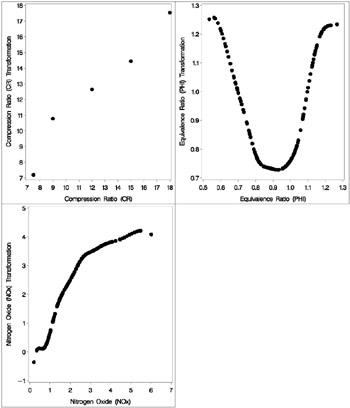
In this example, the MORALS algorithm is applied to data from an experiment in which nitrogen oxide emissions from a single cylinder engine are measured for various combinations of fuel, compression ratio, and equivalence ratio. The data are provided by Brinkman (1981).
The equivalence ratio and nitrogen oxide variables are continuous and numeric, so spline transformations of these variables are requested. Each spline is degree three with nine knots (one at each decile) in order to allow PROC TRANSREG a great deal of freedom in finding transformations. The compression ratio variable has only five discrete values, so an optimal scoring is requested. The character variable Fuel is nominal, so it is designated as a classification variable. No monotonicity constraints are placed on any of the transformations. Observations with missing values are excluded with the NOMISS a-option .
The squared multiple correlation for the initial model is less than 0.25. PROC TRANSREG increases the R 2 to over 0.95 by transforming the variables. The transformation plots show how each variable is transformed. The transformation of compression ratio ( TCpRatio ) is nearly linear. The transformation of equivalence ratio ( TEqRatio ) is nearly parabolic . It can be seen from this plot that the optimal transformation of equivalence ratio is nearly uncorrelated with the original scoring. This suggests that the large increase in R 2 is due to this transformation. The transformation of nitrogen oxide ( TNOx ) is something like a log transformation.
These results suggest the parametric model
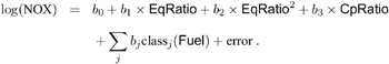
You can perform this analysis with PROC TRANSREG using the following MODEL statement:
model log(NOx)= psp(EqRatio / deg=2) identity(CpRatio) class(Fuel / zero=first);
The LOG transformation computes the natural log. The PSPLINE expansion expands EqRatio into a linear term, EqRatio , and a squared term, EqRatio 2 . A linear transformation of CpRatio and a dummy variable expansion of Fuel is requested with the first level as the reference level. These should provide a good parametric operationalization of the optimal transformations. The final model has an R 2 of 0.91 (smaller than before since the model uses fewer degrees of freedom, but still quite good).
The following statements produce Output 75.4.1 through Output 75.4.2:
| |
Gasoline Example Iteratively Estimate NOx, CPRATIO and EQRATIO The TRANSREG Procedure Dependent Variable Spline(NOx) Nitrogen Oxide (NOx) Class Level Information Class Levels Values Fuel 6 82rongas 94%Eth Ethanol Gasohol Indolene Methanol Number of Observations Read 171 Number of Observations Used 169 TRANSREG MORALS Algorithm Iteration History for Spline(NOx) Iteration Average Maximum Criterion Number Change Change R-Square Change Note ------------------------------------------------------------------------- 0 0.48074 3.86778 0.24597 1 0.00000 0.00000 0.95865 0.71267 Converged Algorithm converged. The TRANSREG Procedure Hypothesis Tests for Spline(NOx) Nitrogen Oxide (NOx) Univariate ANOVA Table Based on the Usual Degrees of Freedom Sum of Mean Source DF Squares Square F Value Liberal p Model 21 326.0946 15.52831 162.27 >= <.0001 Error 147 14.0674 0.09570 Corrected Total 168 340.1619 The above statistics are not adjusted for the fact that the dependent variable was transformed and so are generally liberal. Root MSE 0.30935 R-Square 0.9586 Dependent Mean 2.34593 Adj R-Sq 0.9527 Coeff Var 13.18661 Gasoline Example Iteratively Estimate NOx, CPRATIO and EQRATIO The TRANSREG Procedure Adjusted Multivariate ANOVA Table Based on the Usual Degrees of Freedom Dependent Variable Scoring Parameters=12 S=12 M=4 N=67 Statistic Value F Value Num DF Den DF p Wilks' Lambda 0.041355 2.05 252 1455 <= <.0001 Pillai's Trace 0.958645 0.61 252 1764 <= 1.0000 Hotelling-Lawley Trace 23.18089 12.35 252 945.01 <= <.0001 Roy's Greatest Root 23.18089 162.27 21 147 >= <.0001 The Wilks' Lambda, Pillai's Trace, and Hotelling-Lawley Trace statistics are a conservative adjustment of the normal statistics. Roy's Greatest Root is liberal. These statistics are normally defined in terms of the squared canonical correlations which are the eigenvalues of the matrix H*inv(H+E). Here the R-Square is used for the first eigenvalue and all other eigenvalues are set to zero since only one linear combination is used. Degrees of freedom are computed assuming all linear combinations contribute to the Lambda and Trace statistics, so the F tests for those statistics are conservative. The p values for the liberal and conservative statistics provide approximate lower and upper bounds on p. A liberal test statistic with conservative degrees of freedom and a conservative test statistic with liberal degrees of freedom yield at best an approximate p value, which is indicated by a "~" before the p value.
| |
| |
| |
title 'Gasoline Example'; data Gas; input Fuel :. CpRatio EqRatio NOx @@; label Fuel = 'Fuel' CpRatio = 'Compression Ratio (CR)' EqRatio = 'Equivalence Ratio (PHI)' NOx = 'Nitrogen Oxide (NOx)'; datalines; Ethanol 12.0 0.907 3.741 Ethanol 12.0 0.761 2.295 Ethanol 12.0 1.108 1.498 Ethanol 12.0 1.016 2.881 Ethanol 12.0 1.189 0.760 Ethanol 9.0 1.001 3.120 Ethanol 9.0 1.231 0.638 Ethanol 9.0 1.123 1.170 Ethanol 12.0 1.042 2.358 Ethanol 12.0 1.215 0.606 Ethanol 12.0 0.930 3.669 Ethanol 12.0 1.152 1.000 Ethanol 15.0 1.138 0.981 Ethanol 18.0 0.601 1.192 Ethanol 7.5 0.696 0.926 Ethanol 12.0 0.686 1.590 Ethanol 12.0 1.072 1.806 Ethanol 15.0 1.074 1.962 Ethanol 15.0 0.934 4.028 Ethanol 9.0 0.808 3.148 Ethanol 9.0 1.071 1.836 Ethanol 7.5 1.009 2.845 Ethanol 7.5 1.142 1.013 Ethanol 18.0 1.229 0.414 Ethanol 18.0 1.175 0.812 Ethanol 15.0 0.568 0.374 Ethanol 15.0 0.977 3.623 Ethanol 7.5 0.767 1.869 Ethanol 7.5 1.006 2.836 Ethanol 9.0 0.893 3.567 Ethanol 15.0 1.152 0.866 Ethanol 15.0 0.693 1.369 Ethanol 15.0 1.232 0.542 Ethanol 15.0 1.036 2.739 Ethanol 15.0 1.125 1.200 Ethanol 9.0 1.081 1.719 Ethanol 9.0 0.868 3.423 Ethanol 7.5 0.762 1.634 Ethanol 7.5 1.144 1.021 Ethanol 7.5 1.045 2.157 Ethanol 18.0 0.797 3.361 Ethanol 18.0 1.115 1.390 Ethanol 18.0 1.070 1.947 Ethanol 18.0 1.219 0.962 Ethanol 9.0 0.637 0.571 Ethanol 9.0 0.733 2.219 Ethanol 9.0 0.715 1.419 Ethanol 9.0 0.872 3.519 Ethanol 7.5 0.765 1.732 Ethanol 7.5 0.878 3.206 Ethanol 7.5 0.811 2.471 Ethanol 15.0 0.676 1.777 Ethanol 18.0 1.045 2.571 Ethanol 18.0 0.968 3.952 Ethanol 15.0 0.846 3.931 Ethanol 15.0 0.684 1.587 Ethanol 7.5 0.729 1.397 Ethanol 7.5 0.911 3.536 Ethanol 7.5 0.808 2.202 Ethanol 7.5 1.168 0.756 Indolene 7.5 0.831 4.818 Indolene 7.5 1.045 2.849 Indolene 7.5 1.021 3.275 Indolene 7.5 0.970 4.691 Indolene 7.5 0.825 4.255 Indolene 7.5 0.891 5.064 Indolene 7.5 0.710 2.118 Indolene 7.5 0.801 4.602 Indolene 7.5 1.074 2.286 Indolene 7.5 1.148 0.970 Indolene 7.5 1.000 3.965 Indolene 7.5 0.928 5.344 Indolene 7.5 0.767 3.834 Ethanol 7.5 0.749 1.620 Ethanol 7.5 0.892 3.656 Ethanol 7.5 1.002 2.964 82rongas 7.5 0.873 6.021 82rongas 7.5 0.987 4.467 82rongas 7.5 1.030 3.046 82rongas 7.5 1.101 1.596 82rongas 7.5 1.173 0.835 82rongas 7.5 0.931 5.498 82rongas 7.5 0.822 5.470 82rongas 7.5 0.749 4.084 82rongas 7.5 0.625 0.716 94%Eth 7.5 0.818 2.382 94%Eth 7.5 1.128 1.004 94%Eth 7.5 1.191 0.623 94%Eth 7.5 1.132 1.030 94%Eth 7.5 0.993 2.593 94%Eth 7.5 0.866 2.699 94%Eth 7.5 0.910 3.177 94%Eth 12.0 1.139 1.151 94%Eth 12.0 1.267 0.474 94%Eth 12.0 1.017 2.814 94%Eth 12.0 0.954 3.308 94%Eth 12.0 0.861 3.031 94%Eth 12.0 1.034 2.537 94%Eth 12.0 0.781 2.403 94%Eth 12.0 1.058 2.412 94%Eth 12.0 0.884 2.452 94%Eth 12.0 0.766 1.857 94%Eth 7.5 1.193 0.657 94%Eth 7.5 0.885 2.969 94%Eth 7.5 0.915 2.670 Ethanol 18.0 0.812 3.760 Ethanol 18.0 1.230 0.672 Ethanol 18.0 0.804 3.677 Ethanol 18.0 0.712 . Ethanol 12.0 0.813 3.517 Ethanol 12.0 1.002 3.290 Ethanol 9.0 0.696 1.139 Ethanol 9.0 1.199 0.727 Ethanol 9.0 1.030 2.581 Ethanol 15.0 0.602 0.923 Ethanol 15.0 0.694 1.527 Ethanol 15.0 0.816 3.388 Ethanol 15.0 0.896 . Ethanol 15.0 1.037 2.085 Ethanol 15.0 1.181 0.966 Ethanol 7.5 0.899 3.488 Ethanol 7.5 1.227 0.754 Indolene 7.5 0.701 1.990 Indolene 7.5 0.807 5.199 Indolene 7.5 0.902 5.283 Indolene 7.5 0.997 3.752 Indolene 7.5 1.224 0.537 Indolene 7.5 1.089 1.640 Ethanol 9.0 1.180 0.797 Ethanol 7.5 0.795 2.064 Ethanol 18.0 0.990 3.732 Ethanol 18.0 1.201 0.586 Methanol 7.5 0.975 2.941 Methanol 7.5 1.089 1.467 Methanol 7.5 1.150 0.934 Methanol 7.5 1.212 0.722 Methanol 7.5 0.859 2.397 Methanol 7.5 0.751 1.461 Methanol 7.5 0.720 1.235 Methanol 7.5 1.090 1.347 Methanol 7.5 0.616 0.344 Gasohol 7.5 0.712 2.209 Gasohol 7.5 0.771 4.497 Gasohol 7.5 0.959 4.958 Gasohol 7.5 1.042 2.723 Gasohol 7.5 1.125 1.244 Gasohol 7.5 1.097 1.562 Gasohol 7.5 0.984 4.468 Gasohol 7.5 0.928 5.307 Gasohol 7.5 0.889 5.425 Gasohol 7.5 0.827 5.330 Gasohol 7.5 0.674 1.448 Gasohol 7.5 1.031 3.164 Methanol 7.5 0.871 3.113 Methanol 7.5 1.026 2.551 Methanol 7.5 0.598 0.204 Indolene 7.5 0.973 5.055 Indolene 7.5 0.980 4.937 Indolene 7.5 0.665 1.561 Ethanol 7.5 0.629 0.561 Ethanol 9.0 0.608 0.563 Ethanol 12.0 0.584 0.678 Ethanol 15.0 0.562 0.370 Ethanol 18.0 0.535 0.530 94%Eth 7.5 0.674 0.900 Gasohol 7.5 0.645 1.207 Ethanol 18.0 0.655 1.900 94%Eth 7.5 1.022 2.787 94%Eth 7.5 0.790 2.645 94%Eth 7.5 0.720 1.475 94%Eth 7.5 1.075 2.147 ; *---Fit the Nonparametric Model---; proc transreg data=Gas dummy test nomiss; model spline(NOx / nknots=9)=spline(EqRatio / nknots=9) opscore(CpRatio) class(Fuel / zero=first); title2 'Iteratively Estimate NOx, CPRATIO and EQRATIO'; output out=Results; run; *---Plot the Results---; goptions goutmode=replace nodisplay; %let opts = haxis=axis2 vaxis=axis1 frame cframe=ligr; * Depending on your goptions, these plot options may work better: * %let opts = haxis=axis2 vaxis=axis1 frame; proc gplot data=Results; title; axis1 minor=none label=(angle=90 rotate=0); axis2 minor=none; symbol1 color=blue v=dot i=none; plot TCpRatio*CpRatio / &opts name='tregex1'; plot TEqRatio*EqRatio / &opts name='tregex2'; plot TNOx*NOx / &opts name='tregex3'; run; quit; goptions display; proc greplay nofs tc=sashelp.templt template=l2r2; igout gseg; treplay 1:tregex1 2:tregex3 3:tregex2; run; quit; *-Fit the Parametric Model Suggested by the Nonparametric Analysis-; proc transreg data=Gas dummy ss2 short nomiss; title 'Gasoline Example'; title2 'Now fit log(NOx) = b0 + b1*EqRatio + b2*EqRatio**2 +'; title3 'b3*CpRatio + Sum b(j)*Fuel(j) + Error'; model log(NOx)= pspline(EqRatio / deg=2) identity(CpRatio) class(Fuel / zero=first); output out=Results2; run;
| |
Gasoline Example Now fit log(NOx) = b0 + b1*EqRatio + b2*EqRatio**2 + b3*CpRatio + Sum b(j)*Fuel(j) + Error The TRANSREG Procedure Dependent Variable Log(NOx) Nitrogen Oxide (NOx) Class Level Information Class Levels Values Fuel 6 82rongas 94%Eth Ethanol Gasohol Indolene Methanol Number of Observations Read 171 Number of Observations Used 169 Log(NOx) Algorithm converged. The TRANSREG Procedure Hypothesis Tests for Log(NOx) Nitrogen Oxide (NOx) Univariate ANOVA Table Based on the Usual Degrees of Freedom Sum of Mean Source DF Squares Square F Value Pr > F Model 8 79.33838 9.917298 213.09 <.0001 Error 160 7.44659 0.046541 Corrected Total 168 86.78498 Root MSE 0.21573 R-Square 0.9142 Dependent Mean 0.63130 Adj R-Sq 0.9099 Coeff Var 34.17294 Univariate Regression Table Based on the Usual Degrees of Freedom Type II Sum of Mean Variable DF Coefficient Squares Square F Value Pr > F Label Intercept 1 14.586532 49.9469 49.9469 1073.18 <.0001 Intercept Pspline.EqRatio_1 1 35.102914 62.7478 62.7478 1348.22 <.0001 Equivalence Ratio (PHI) 1 Pspline.EqRatio_2 1 19.386468 64.6430 64.6430 1388.94 <.0001 Equivalence Ratio (PHI) 2 Identity(CpRatio) 1 0.032058 1.4445 1.4445 31.04 <.0001 Compression Ratio (CR) Class.Fuel94_Eth 1 0.449583 1.3158 1.3158 28.27 <.0001 Fuel 94%Eth Class.FuelEthanol 1 0.414242 1.2560 1.2560 26.99 <.0001 Fuel Ethanol Class.FuelGasohol 1 0.016719 0.0015 0.0015 0.03 0.8584 Fuel Gasohol Class.FuelIndolene 1 0.001572 0.0000 0.0000 0.00 0.9853 Fuel Indolene Class.FuelMethanol 1 0.580133 1.7219 1.7219 37.00 <.0001 Fuel Methanol
| |
Example 75.5. Preference Mapping of Cars Data
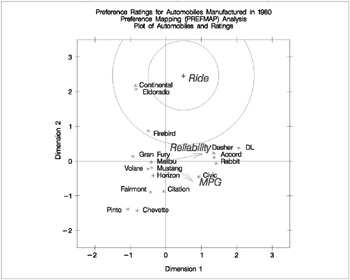
This example uses PROC TRANSREG to perform a preference mapping (PREFMAP) analysis (Carroll 1972) of car preference data after a PROC PRINQUAL principal component analysis. The PREFMAP analysis is a response surface regression that locates ideal points for each dependent variable in a space defined by the independent variables.
The data are ratings obtained from 25 judges of their preference for each of 17 automobiles. The ratings were made on a zero (very weak preference) to nine (very strong preference) scale. These judgments were made in 1980 about that year's products. There are two character variables that indicate the manufacturer and model of the automobile. The data set also contains three ratings: miles per gallon ( MPG ), projected reliability ( Reliability ), and quality of the ride ( Ride ). These ratings are on a one (bad) to five (good) scale. PROC PRINQUAL creates an OUT= data set containing standardized principal component scores ( Prin1 and Prin2 ), along with the ID variables MODEL, MPG , Reliability ,and Ride .
The first PROC TRANSREG step fits univariate regression models for MPG and Reliability . All variables are designated IDENTITY. A vector drawn in the plot of Prin1 and Prin2 from the origin to the point defined by an attribute's regression coefficients approximately shows how the cars differ on that attribute. Refer to Carroll (1972) for more information. The Prin1 and Prin2 columns of the TResult1 OUT= data set contain the car coordinates ( _Type_ ='SCORE' observations) and endpoints of the MPG and Reliability vectors ( _Type_ ='M COEFFI' observations).
The second PROC TRANSREG step fits a univariate regression model with Ride designated IDENTIY, and Prin1 and Prin2 designated POINT. The POINT expansion creates an additional independent variable _ISSQ_ , which contains the sum of Prin1 squared and Prin2 squared. The OUT= data set TResult2 contains no _Type_ ='SCORE' observations, only ideal point ( _Type_ ='M POINT') coordinates for Ride . The coordinates of both the vectors and the ideal points are output by specifying COORDINATES in the OUTPUT statement in PROC TRANSREG.
A vector model is used for MPG and Reliability because perfectly efficient and reliable cars do not exist in the data set. The ideal points for MPG and Reliability are far removed from the plot of the cars. It is more likely that an ideal point for quality of the ride is in the plot, so an ideal point model is used for the ride variable. Refer to Carroll (1972) and Schiffman, Reynolds, and Young (1981) for discussions of the vector model and point models (including the EPOINT and QPOINT versions of the point model that are not used in this example).
The final DATA step combines the two output data sets and creates a data set suitable for the %PLOTIT macro. (For information on the %PLOTIT macro, see Appendix B, 'Using the %PLOTIT Macro.') The plot contains one point per car and one point for each of the three ratings. The % PLOTIT macro options specify the input data set, how to handle anti-ideal points (described later), and where to draw horizontal and vertical reference lines. The DATATYPE= option specifies that the input data set contains results of a PREFMAP vector model and a PREFMAP ideal point model.
This instructs the macro to draw vectors to _Type_ ='M COEFFI' observations and circles around _Type_ ='M POINT' observations.
An unreliable to reliable direction extends from the left and slightly below the origin to the right and slightly above the origin. The Japanese and European Cars are rated, on the average, as more reliable. A low MPG to good MPG direction extends from the top left of the plot to the bottom right. The smaller cars, on the average, get better gas mileage. The ideal point for Ride is in the top, just right of the center of the plot. Cars near the Ride ideal point tend to have a better ride than cars far away. It can be seen from the iteration history tables that none of these ratings perfectly fits the model, so all of the interpretations are approximate.
The Ride point is a 'negative-negative' ideal point. The point models assume that small ratings mean the object (car) is similar to the rating name and large ratings imply dissimilarity to the rating name. Because the opposite scoring is used, the interpretation of the Ride point must be reversed to a negative ideal point (bad ride). However, the coefficient for the _ISSQ_ variable is negative, so the interpretation is reversed again, back to the original interpretation. Anti-ideal points are taken care of in the %PLOTIT macro. Specify ANTIIDEA=1 when large values are positive or ideal and ANTIIDEA=-1 when small values are positive or ideal.
The following statements produce Output 75.5.1 through Output 75.5.2:
title 'Preference Ratings for Automobiles Manufactured in 1980'; data CarPreferences; input Make $ 1-10 Model $ 12-22 @25 (Judge1-Judge25) (1.) MPG Reliability Ride; datalines; Cadillac Eldorado 8007990491240508971093809 3 2 4 Chevrolet Chevette 0051200423451043003515698 5 3 2 Chevrolet Citation 4053305814161643544747795 4 1 5 Chevrolet Malibu 6027400723121345545668658 3 3 4 Ford Fairmont 2024006715021443530648655 3 3 4 Ford Mustang 5007197705021101850657555 3 2 2 Ford Pinto 0021000303030201500514078 4 1 1 Honda Accord 5956897609699952998975078 5 5 3 Honda Civic 4836709507488852567765075 5 5 3 Lincoln Continental 7008990592230409962091909 2 4 5 Plymouth Gran Fury 7006000434101107333458708 2 1 5 Plymouth Horizon 3005005635461302444675655 4 3 3 Plymouth Volare 4005003614021602754476555 2 1 3 Pontiac Firebird 0107895613201206958265907 1 1 5 Volkswagen Dasher 4858696508877795377895000 5 3 4 Volkswagen Rabbit 4858509709695795487885000 5 4 3 Volvo DL 9989998909999987989919000 4 5 5 ; *---Compute Coordinates for a 2-Dimensional Scatter Plot of Cars---; proc prinqual data=CarPreferences out=PResults(drop=Judge1-Judge25) n=2 replace standard scores; id Model MPG Reliability Ride; transform identity(Judge1-Judge25); title2 'Multidimensional Preference (MDPREF) Analysis'; run; *---Compute Endpoints for MPG and Reliability Vectors---; proc transreg data=PResults; Model identity(MPG Reliability)=identity(Prin1 Prin2); output tstandard=center coordinates replace out=TResult1; id Model; title2 'Preference Mapping (PREFMAP) Analysis'; run; *---Compute Ride Ideal Point Coordinates---; proc transreg data=PResults; Model identity(Ride)=point(Prin1 Prin2); output tstandard=center coordinates replace noscores out=TResult2; id Model; run; proc print; run; *---Combine Data Sets and Plot the Results---; data plot; title3 'Plot of Automobiles and Ratings'; set Tresult1 Tresult2; run; %plotit(data=plot, datatype=vector ideal, antiidea=1, href=0, vref=0);
| |
| |
| |
Preference Ratings for Automobiles Manufactured in 1980 Multidimensional Preference (MDPREF) Analysis The PRINQUAL Procedure PRINQUAL MTV Algorithm Iteration History Iteration Average Maximum Proportion Criterion Number Change Change of Variance Change Note ---------------------------------------------------------------------------- 1 0.00000 0.00000 0.66946 Converged Algorithm converged. WARNING: The number of observations is less than or equal to the number of variables. WARNING: Multiple optimal solutions may exist. Preference Ratings for Automobiles Manufactured in 1980 Preference Mapping (PREFMAP) Analysis The TRANSREG Procedure TRANSREG Univariate Algorithm Iteration History for Identity(MPG) Iteration Average Maximum Criterion Number Change Change R-Square Change Note ------------------------------------------------------------------------- 1 0.00000 0.00000 0.57197 Converged Algorithm converged. Preference Ratings for Automobiles Manufactured in 1980 Preference Mapping (PREFMAP) Analysis The TRANSREG Procedure TRANSREG Univariate Algorithm Iteration History for Identity(Reliability) Iteration Average Maximum Criterion Number Change Change R-Square Change Note ------------------------------------------------------------------------- 1 0.00000 0.00000 0.50859 Converged Algorithm converged. Preference Ratings for Automobiles Manufactured in 1980 Preference Mapping (PREFMAP) Analysis The TRANSREG Procedure TRANSREG Univariate Algorithm Iteration History for Identity(Ride) Iteration Average Maximum Criterion Number Change Change R-Square Change Note ------------------------------------------------------------------------- 1 0.00000 0.00000 0.37797 Converged Algorithm converged. Preference Ratings for Automobiles Manufactured in 1980 Preference Mapping (PREFMAP) Analysis Obs _TYPE_ _NAME_ Ride Intercept Prin1 Prin2 _ISSQ_ Model 1 M POINT Ride . . 0.49461 2.46539 -0.17448 Ride
| |
Example 75.6. Box Cox
This example illustrates finding a Box-Cox transformation (see the 'Box-Cox Transformations' section on page 4595) of some artificial data. Data were generated from the model
y = e x + ˆˆ
where ˆˆ ~ N(0,1). The transformed data can be fit with a linear model
log( y ) = x + ˆˆ
These statements produce Output 75.6.1.
title 'Basic Box-Cox Example'; data x; do x = 1 to 8 by 0.025; y = exp(x + normal(7)); output; end; run; proc transreg data=x ss2 details; title2 'Defaults'; model boxcox(y) = identity(x); run;
| |
Basic Box-Cox Example 88 Defaults The TRANSREG Procedure Transformation Information for BoxCox(y) Lambda R-Square Log Like 3.00 0.03 4601.01 2.75 0.04 4266.08 2.50 0.04 3934.11 2.25 0.05 3605.75 2.00 0.06 3281.88 1.75 0.07 2963.74 1.50 0.10 2653.14 1.25 0.14 2352.72 1.00 0.21 2066.32 0.75 0.34 1799.25 0.50 0.52 1558.55 0.25 0.71 1360.28 0.00 + 0.79 1275.31 < 0.25 0.70 1382.62 0.50 0.51 1589.03 0.75 0.34 1834.53 1.00 0.22 2105.88 1.25 0.15 2397.35 1.50 0.11 2704.64 1.75 0.08 3024.24 2.00 0.06 3353.38 2.25 0.05 3689.91 2.50 0.04 4032.18 2.75 0.03 4378.97 3.00 0.03 4729.37 < - Best Lambda * - Confidence Interval + - Convenient Lambda
| |
PROC TRANSREG correctly selects the log transformation » = 0, with a narrow confidence interval. The maximum of the log likelihood function is flagged with the less-than sign (<), and the convenient power parameter of » = 0 in the confidence interval is flagged by the plus sign (+). The rest of the output is shown next in Output 75.6.2.
| |
Basic Box-Cox Example 89 Defaults The TRANSREG Procedure Dependent Variable BoxCox(y) Number of Observations Read 281 Number of Observations Used 281 TRANSREG Univariate Algorithm Iteration History for BoxCox(y) Iteration Average Maximum Criterion Number Change Change R-Square Change Note ------------------------------------------------------------------------- 1 0.00000 0.00000 0.79064 Converged Algorithm converged. Model Statement Specification Details Type DF Variable Description Value Dep 1 BoxCox(y) Lambda Used 0 Lambda 0 Log Likelihood -1275.3 Conv. Lambda 0 Conv. Lambda LL -1275.3 CI Limit -1277.2 Alpha 0.05 Ind 1 Identity(x) DF 1 The TRANSREG Procedure Hypothesis Tests for BoxCox(y) Univariate ANOVA Table Based on the Usual Degrees of Freedom Sum of Mean Source DF Squares Square F Value Liberal p Model 1 1145.884 1145.884 1053.66 >= <.0001 Error 279 303.421 1.088 Corrected Total 280 1449.305 The above statistics are not adjusted for the fact that the dependent variable was transformed and so are generally liberal. Root MSE 1.04285 R-Square 0.7906 Dependent Mean 4.49653 Adj R-Sq 0.7899 Coeff Var 23.19225 Lambda 0.0000 Univariate Regression Table Based on the Usual Degrees of Freedom Type II Sum of Mean Variable DF Coefficient Squares Square F Value Liberal p Intercept 1 0.01551366 0.01 0.01 0.01 >= 0.9185 Identity(x) 1 0.99578183 1145.88 1145.88 1053.66 >= <.0001 The above statistics are not adjusted for the fact that the dependent variable was transformed and so are generally liberal.
| |
This next example uses several options. The LAMBDA= option specifies power parameters sparsely from -2 to -0.5 and 0.5 to 2 just to get the general shape of the log likelihood function in that region. Between -0.5 and 0.5, more power parameters are tried. The CONVENIENT option is specified so that if a power parameter like » = 1 or » = 0 is found in the confidence interval, it will be used instead of the optimal power parameter. PARAMETER=2 is specified to add 2 to each y before performing the transformations. ALPHA=0.00001 specifiesawideconfidence interval.
These statements produce Output 75.6.3.
| |
Basic Box-Cox Example 90 Several Options Demonstrated The TRANSREG Procedure Transformation Information for BoxCox(y) Lambda R-Square Log Like 2.000 0.22 2583.73 1.000 0.45 1779.35 0.500 0.67 1439.82 0.450 0.70 1410.51 0.400 0.72 1382.74 0.350 0.74 1356.92 0.300 0.76 1333.59 0.250 0.77 1313.42 0.200 0.79 1297.21 0.150 0.79 1285.83 * 0.100 0.80 1280.09 < 0.050 0.80 1280.63 * 0.000 + 0.79 1287.71 * 0.050 0.78 1301.19 0.100 0.76 1320.56 0.150 0.74 1345.09 0.200 0.72 1373.99 0.250 0.69 1406.51 0.300 0.65 1442.02 0.350 0.62 1480.02 0.400 0.58 1520.13 0.450 0.54 1562.05 0.500 0.50 1605.57 1.000 0.22 2105.88 2.000 0.06 3320.36 < - Best Lambda * - Confidence Interval + - Convenient Lambda
| |
proc transreg data=x ss2 details; title2 'Several Options Demonstrated'; model boxcox(y / lambda= 2 1 0.5 to 0.5 by 0.05 1 2 convenient parameter=2 alpha=0.00001) = identity(x); run;
The results show that the optimal power parameter is -0.1 but 0 is in the confidence interval, hence a log transformation is chosen . The rest of the output is shown next in Output 75.6.4.
| |
Basic Box-Cox Example 91 Several Options Demonstrated The TRANSREG Procedure Dependent Variable BoxCox(y) Number of Observations Read 281 Number of Observations Used 281 TRANSREG Univariate Algorithm Iteration History for BoxCox(y) Iteration Average Maximum Criterion Number Change Change R-Square Change Note ------------------------------------------------------------------------- 1 0.00000 0.00000 0.79238 Converged Algorithm converged. Model Statement Specification Details Type DF Variable Description Value Dep 1 BoxCox(y) Lambda Used 0 Lambda 0.1 Log Likelihood 1280.1 Conv. Lambda 0 Conv. Lambda LL 1287.7 CI Limit 1289.9 Alpha 0.00001 Parameter 2 Options Convenient Lambda Used Ind 1 Identity(x) DF 1 Basic Box-Cox Example 92 Several Options Demonstrated The TRANSREG Procedure The TRANSREG Procedure Hypothesis Tests for BoxCox(y) Univariate ANOVA Table Based on the Usual Degrees of Freedom Sum of Mean Source DF Squares Square F Value Liberal p Model 1 999.438 999.4381 1064.82 >= <.0001 Error 279 261.868 0.9386 Corrected Total 280 1261.306 The above statistics are not adjusted for the fact that the dependent variable was transformed and so are generally liberal. Root MSE 0.96881 R-Square 0.7924 Dependent Mean 4.61429 Adj R-Sq 0.7916 Coeff Var 20.99591 Lambda 0.0000 Univariate Regression Table Based on the Usual Degrees of Freedom Type II Sum of Mean Variable DF Coefficient Squares Square F Value Liberal p Intercept 1 0.42939328 8.746 8.746 9.32 >= 0.0025 Identity(x) 1 0.92997620 999.438 999.438 1064.82 >= <.0001 The above statistics are not adjusted for the fact that the dependent variable was transformed and so are generally liberal.
| |
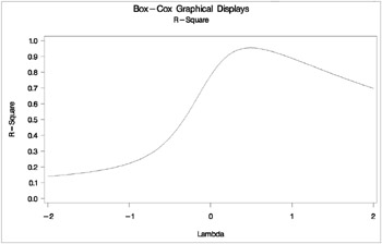
The next part of this example shows how to make graphical displays of the Box-Cox transformation results. Plots include the log likelihood function with the confidence interval, root mean squared error as a function of the power parameter, R 2 as a function of the power parameter, the Box-Cox transformation of the variable y , the original scatter plot based on the untransformed data, and the new scatter plot based on the transformed data. Also, a condensed version of the log likelihood table with the confidence interval is printed. Here are the data.
title h=1 'Box-Cox Graphical Displays'; data x; input y x @@; datalines; 10.0 3.0 72.6 8.3 59.7 8.1 20.1 4.8 90.1 9.8 1.1 0.9 78.2 8.5 87.4 9.0 9.5 3.4 0.1 1.4 0.1 1.1 42.5 5.1 57.0 7.5 9.9 1.9 0.5 1.0 121.1 9.9 37.5 5.9 49.5 6.7 8.3 1.8 0.6 1.8 53.0 6.7 112.8 10.0 40.7 6.4 5.1 2.4 73.3 9.5 122.4 9.9 87.2 9.4 121.2 9.9 23.1 4.3 7.1 3.5 12.4 3.3 5.6 2.7 113.0 9.6 110.5 10.0 3.1 1.5 52.4 7.9 80.4 8.1 0.6 1.6 115.1 9.1 15.9 3.1 56.5 7.3 85.4 9.8 32.5 5.8 43.0 6.2 0.1 0.8 21.8 5.2 15.2 3.5 5.2 3.0 0.2 0.8 73.5 8.2 4.9 3.2 0.2 0.3 69.0 9.2 3.6 3.5 0.2 0.9 101.3 9.9 10.0 3.7 16.9 3.0 11.2 5.0 0.2 0.4 80.8 9.4 24.9 5.7 113.5 9.7 6.2 2.1 12.5 3.2 4.8 1.8 80.1 8.3 26.4 4.8 13.4 3.8 99.8 9.7 44.1 6.2 15.3 3.8 2.2 1.5 10.3 2.7 13.8 4.7 38.6 4.5 79.1 9.8 33.6 5.8 9.1 4.5 89.3 9.1 5.5 2.6 20.0 4.8 2.9 2.9 82.9 8.4 7.0 3.5 14.5 2.9 16.0 3.7 29.3 6.1 48.9 6.3 1.6 1.9 34.7 6.2 33.5 6.5 26.0 5.6 12.7 3.1 0.1 0.3 15.4 4.2 2.6 1.8 58.6 7.9 81.2 8.1 37.2 6.9
The TRANSREG procedure is run to find the Box-Cox transformation. The lambda list is -2 TO 2 BY 0.01, which produces 401 lambdas. This many power parameters makes a nice graphical display with plenty of detail around the confidence interval. However, 401 values is a lot to print, so for this reason, the usual Box-Cox transformation information table is excluded from the printed output. Instead, it is output to a SAS data set using ODS so a sample of it can be printed. Just the confidence interval and the rows corresponding to power parameters that are multiples of 0.5 are printed. Null labels are provided for the columns that need to be printed without headers. The details table is also output to a SAS data set using ODS, since it contains information that will be incorporated into some of the plots. These statements produce Output 75.6.5.
| |
Box-Cox Graphical Displays 93 The TRANSREG Procedure TRANSREG Univariate Algorithm Iteration History for BoxCox(y) Iteration Average Maximum Criterion Number Change Change R-Square Change Note ------------------------------------------------------------------------- 1 0.00000 0.00000 0.95396 Converged Algorithm converged. Model Statement Specification Details Type DF Variable Description Value Dep 1 BoxCox(y) Lambda Used 0.5 Lambda 0.46 Log Likelihood 167.0 Conv. Lambda 0.5 Conv. Lambda LL 168.3 CI Limit 169.0 Alpha 0.05 Options Convenient Lambda Used Ind 1 Identity(x) DF 1 Box-Cox Graphical Displays 94 Confidence Interval Dependent Lambda R-Square Log Like BoxCox(y) 2.00 0.14 1030.56 BoxCox(y) 1.50 0.17 810.50 BoxCox(y) 1.00 0.22 602.53 BoxCox(y) 0.50 0.39 415.56 BoxCox(y) 0.00 0.78 257.92 BoxCox(y) 0.41 0.95 168.40 * BoxCox(y) 0.42 0.95 167.86 * BoxCox(y) 0.43 0.95 167.46 * BoxCox(y) 0.44 0.95 167.19 * BoxCox(y) 0.45 0.95 167.05 * BoxCox(y) 0.46 0.95 167.04 < BoxCox(y) 0.47 0.95 167.16 * BoxCox(y) 0.48 0.95 167.41 * BoxCox(y) 0.49 0.95 167.79 * BoxCox(y) 0.50 + 0.95 168.28 * BoxCox(y) 0.51 0.95 168.89 * BoxCox(y) 1.00 0.89 253.09 BoxCox(y) 1.50 0.79 345.35 BoxCox(y) 2.00 0.70 435.01
| |
* Fit Box-Cox model, output results to output data sets; ods output boxcox=b details=d; ods exclude boxcox; proc transreg details data=x; model boxcox(y / convenient lambda= 2 to 2 by 0.01) = identity(x); output out=trans; run; proc print noobs label data=b(drop=rmse); title2 'Confidence Interval'; where ci ne ' ' or abs(lambda - round(lambda, 0.5)) < 1e-6; label convenient = '00'x ci = '00'x; run; ; These next steps extract information from the Box-Cox transformation and details tables and store the information in macro variables. The confidence interval limit from the details table provides a vertical axis reference line for the log likelihood plot. The convenient power parameter ('Lambda Used') is extracted from the footnote. The confidence interval is extracted from the confidence interval observations of the Box-Cox transformation table and will be used in the footnote and for horizontal axis reference lines in the log likelihood plot.
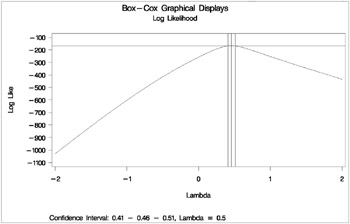
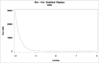
* Store values for reference lines; data _null_; set d; if description = 'CI Limit' then call symput('vref', formattedvalue); if description = 'Lambda Used' then call symput('lambda', formattedvalue); run; data _null_; set b end=eof; where ci ne ' '; if _n_ = 1 then call symput('href1', compress(put(lambda, best12.))); if ci = '<' then call symput('href2', compress(put(lambda, best12.))); if eof then call symput('href3', compress(put(lambda, best12.))); run; These steps plot the log likelihood, root mean square error and R 2 . The input data set is the Box-Cox transformation table, which was output using ODS. These statements produce Output 75.6.6.
| |
| |
* Plot log likelihood, confidence interval; axis1 label=(angle=90 rotate=0) minor=none; axis2 minor=none; proc gplot data=b; title2 'Log Likelihood'; plot loglike * lambda / vref=&vref href=&href1 &href2 &href3 vaxis=axis1 haxis=axis2 frame cframe=ligr; footnote "Confidence Interval: &href1 - &href2 - &href3, " "Lambda = &lambda"; symbol v=none i=spline c=blue; run; footnote; title2 'RMSE'; plot rmse * lambda / vaxis=axis1 haxis=axis2 frame cframe=ligr; run; title2 'R-Square'; plot rsquare * lambda / vaxis=axis1 haxis=axis2 frame cframe=ligr; axis1 order=(0 to 1 by 0.1) label=(angle=90 rotate=0) minor=none; run; quit;
The optimal power parameter is 0.46, but since 0.5 is in the confidence interval, and since the CONVENIENT option was specified, the procedure chooses a square root transformation.
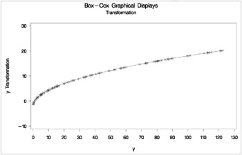
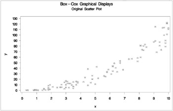
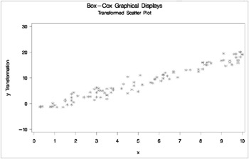
The next steps plot the transformation of Y , the original scatter plot based on the untransformed data, and the new scatter plot based on the transformed data. The results are shown in Output 75.6.7. The input data set is the ordinary output data set from PROC TRANSREG. The transformation of the variable Y by default is Ty .
| |
| |
axis1 label=(angle=90 rotate=0) minor=none; axis2 minor=none; proc gplot data=trans; title2 'Transformation'; symbol i=splines v=star c=blue; plot ty * y / vaxis=axis1 haxis=axis2 frame cframe=ligr; run; title2 'Original Scatter Plot'; symbol i=none v=star c=blue; plot y * x / vaxis=axis1 haxis=axis2 frame cframe=ligr; run; title2 'Transformed Scatter Plot'; symbol i=none v=star c=blue; plot ty * x / vaxis=axis1 haxis=axis2 frame cframe=ligr; run; quit;
The square root transformation makes the scatter plot essentially linear.
[*] In real conjoint experiments, real brand names are used.
[*] In real conjoint experiments, real brand names would be used
EAN: 2147483647
Pages: 132
- ERP Systems Impact on Organizations
- ERP System Acquisition: A Process Model and Results From an Austrian Survey
- Context Management of ERP Processes in Virtual Communities
- Data Mining for Business Process Reengineering
- Relevance and Micro-Relevance for the Professional as Determinants of IT-Diffusion and IT-Use in Healthcare