Syntax

• PROC NLIN < options > ;

  • MODEL dependent=expression ;

  • PARAMETERS parameter=values < , ... , parameter=values > ; other program statements

  • BOUNDS inequality < , ... , inequality > ;

  • BY variables ;

  • DER. parameter=expression ;

  • DER. parameter . parameter=expression ;

  • ID variables ;

  • OUTPUT OUT= SAS-data-set keyword= names < , ... , keyword=names > ;

  • CONTROL variable < =values ><... variable < =values >> ;

A vertical bar () denotes a choice between two specifications. The other program statements are valid SAS expressions that can appear in the DATA step. PROC NLIN enables you to create new variables within the procedure and use them in the nonlinear analysis. The NLIN procedure automatically creates several variables that are also available for use in the analysis. See the section Special Variables beginning on page 3020 for more information. The PROC NLIN, PARMS , and MODEL statements are required.

The statements used in PROC NLIN, in addition to the PROC statement, are as follows :

BOUNDS	constrains the parameter estimates within specified bounds
BY	specifies variables to define subgroups for the analysis
DER	specifies the first or second partial derivatives
ID	specifies additional variables to add to the output data set
MODEL	defines the relationship between the dependent and indep endent variables
OUTPUT	creates an output data set containing statistics for each observation
PARMS	identifies parameters to be estimated and the starting values for each parameter
other program statements	includes assignment statements, ARRAY statements, DO loops , and program control statements

PROC NLIN Statement

• PROC NLIN < options > ;

The PROC NLIN statement invokes the procedure. The following table lists the options available with the PROC NLIN statement. Explanations follow in alphabetical order.

Task	Options
Specify data sets	DATA= OUTEST= SAVE Grid search BEST=
Choose an iteration method	METHOD=
Control step size	MAXSUBIT= NOHALVE RHO= SMETHOD= TAU=
Specify details of iteration	G4 UNCORRECTEDDF SIGSQ=
Minimization Tuning	CONVERGE= CONVERGEOBJ= CONVERGEPARM= SINGULAR= MAXITER=
Modify Amount of Output	HOUGAARD NOITPRINT NOPRINT
List Model Structure	LIST LISTALL LISTCODE LISTDEP LISTDER XREF
Trace Model Execution	FLOW PRINT TRACE

BEST= n

• requests that PROC NLIN display the residual sums of squares only for the best n combinations of possible starting values from the grid. If you do not specify the BEST= option, PROC NLIN displays the residual sum of squares for every combination of possible parameter starting values.

CONVERGE= c

• specifies the convergence criteria for PROC NLIN. For all iterative methods the relative offset convergence measure of Bates and Watts is used by default to determine convergence. This measure is labeled "R" in the Estimation Summary table. The iterations are said to have converged for CONVERGE= c if

  

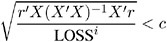
  where r is the residual vector and X is the Jacobian matrix. The default LOSS function is the sum of squared errors (SSE). By default, CONVERGE=10 ^{ˆ’ 5} . The R convergence measure cannot be computed accurately in the special case of a perfect fit (residuals close to zero). When the SSE is less than the value of the SINGULAR= option, convergence is assumed.

CONVERGEOBJ= c

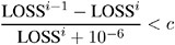
• uses the change in the LOSS function as the convergence criterion. For more details on the LOSS function, see the section Special Variable Used to Determine Convergence Criteria on page 3021. The iterations are said to have converged for CONVERGEOBJ= c if

  

• where LOSS ⁱ is the LOSS for the i th iteration. The default LOSS function is the sum of squared errors (SSE). The constant c should be a small positive number. See the Computational Methods section beginning on page 3024 for more details. If specified, the CONVERGEOBJ= option overrides the default CONVERGE= convergence criterion so that NLIN performs as it did in version 6 releases of the procedure.

CONVERGEPARM= c

• uses the maximum change among parameter estimates as the convergence criterion. The iterations are said to have converged for CONVERGEPARM= c if max

  

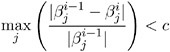
  where is the value of the j th parameter at the i th iteration.

  The default convergence criterion is CONVERGE. If you specify CONVERGEPARM= c , the maximum change in parameters is used as the convergence criterion. If you specify both the CONVERGEOBJ= and CONVERGEPARM= options, PROC NLIN continues to iterate until the decrease in LOSS is sufficiently small (as determined by the CONVERGEOBJ= option) and the maximum change among the parameters is sufficiently small (as determined by the CONVERGEPARM= option).

DATA= SAS-data-set

• specifies the SAS data set containing the data to be analyzed by PROC NLIN. If you omit the DATA= option, the most recently created SAS data set is used.

FLOW

• displays a message for each statement in the model program as it is executed. This debugging option is rarely needed, and it produces large amounts of output.

G4

• uses a Moore-Penrose ( g ₄ ) inverse in parameter estimation. Refer to Kennedy and Gentle (1980) for details.

HOUGAARD

• adds Hougaard s measure of skewness to the parameter estimation table. Computation of the measure requires derivatives (see the section Hougaard s Measure of Skewness on page 3019).

LIST

• displays the model program and variable lists, including the statements added by macros. Note that the expressions displayed by the LIST option do not necessarily represent the way the expression is actually calculated, since intermediate results for common subexpressions can be reused but are shown in expanded form by the LIST option. To see how the expression is actually evaluated, see the description for the LISTCODE option, which follows.

LISTALL

• selects the LIST, LISTDEP, LISTDER, and LISTCODE options.

LISTCODE

• displays the derivative tables and compiled model program code. The LISTCODE option is a debugging feature and is not normally needed.

LISTDEP

• produces a report that lists, for each variable in the model program, the variables that depend on it and on which it depends.

LISTDER

• displays a table of derivatives. The derivatives table lists each nonzero derivative computed for the problem. The derivative listed can be a constant, a variable in the model program, or a special derivative variable created to hold the result of the derivative expression.

MAXITER= i

• limits the number of iterations PROC NLIN performs before it gives up trying to converge. The i value must be a positive integer. By default, MAXITER=100.

MAXSUBIT= i

• places a limit on the number of step halvings. By default, MAXSUBIT=30. The value of MAXSUBIT must be a positive integer.

METHOD=GAUSS MARQUARDT NEWTON GRADIENT

• specifies the iterative method that PROC NLIN uses. The GAUSS, MARQUARDT and NEWTON methods are more robust than the GRADIENT method. If you omit the METHOD= option, METHOD=GAUSS is used. See the Computational Methods section beginning on page 3024 for more information.

NOITPRINT

• suppresses the display of the results of each iteration.

NOHALVE

• removes the restriction that the objective value must decrease at every iteration. Step halving is still used to satisfy BOUNDS and to ensure that the number of observations that can be evaluated does not decrease. NOHALVE is useful for iteratively reweighted least squares problems.

NOPRINT

• suppresses the display of the output. Note that this option temporarily disables the Output Delivery System (ODS). For more information, see Chapter 14, Using the Output Delivery System.

OUTEST= SAS-data-set

• specifies an output data set to contain the parameter estimates produced at each iteration. See the Output Data Sets section on page 3028 for details. If you want to create a permanent SAS data set, you must specify a two-level name . See the chapter SAS Files, in SAS Language Reference: Concepts for more information on permanent SAS data sets.

PRINT

• displays the result of each statement in the program as it is executed. This option produces large amounts of output.

RHO= value

• specifies a value to use in controlling the step-size search. By default, RHO=0.1 except when METHOD=MARQUARDT, in which case RHO=10. See the section Computational Methods beginning on page 3024 for more details.

SAVE

• specifies that, when the iteration limit is exceeded, the parameter estimates from the final iteration are output to the OUTEST= data set. These parameter estimates are located in the observation with _TYPE_ =FINAL. If you omit the SAVE option, the parameter estimates from the final iteration are not output to the data set unless convergence is attained.

SIGSQ= value

• specifies a value to replace the mean square error for computing the standard errors of the estimates. The SIGSQ= option is used with maximum- likelihood estimation.

SINGULAR= s

• specifies the singularity criterion, s , which is the absolute magnitude of the smallest pivot value allowed when inverting the Hessian or approximation to the Hessian. The default value is 1E-8.

SMETHOD=HALVE GOLDEN CUBIC

• specifies the step-size search method that PROC NLIN uses. The default is SMETHOD=HALVE. See the section Computational Methods beginning on page 3024 for details.

TAU= value

• specifies a value to use in controlling the step-size search. By default, TAU=1 except when METHOD=MARQUARDT, in which case TAU=0.01. See the section Computational Methods beginning on page 3024 for details.

TRACE

• displays the result of each operation in each statement in the model program as it is executed, in addition to the information displayed by the FLOW and PRINT options. This debugging option is needed very rarely, and it produces even more output than the FLOW and PRINT options.

XREF

• displays a cross-reference of the variables in the model program showing where each variable is referenced or given a value. The XREF listing does not include derivative variables.

UNCORRECTEDDF

• specifies that no degrees of freedom are lost when a bound is active. When the UNCORRECTEDDF option is not specified, an active bound is treated as if a restriction was applied to the set of parameters so one parameter degree of freedom is deducted.

BOUNDS Statement

• BOUNDS inequality <,..., inequality > ;

The BOUNDS statement restrains the parameter estimates within specified bounds. In each BOUNDS statement, you can specify a series of bounds separated by commas. The series of bounds is applied simultaneously . Each bound contains a list of parameters, an inequality comparison operator, and a value. In a single-bounded expression, these three elements follow one another in the order described. The following are examples of valid single-bounded expressions:

  bounds a1   a10<=20;   bounds c>30;   boundsa b c > 0;  

Multiple-bounded expressions are also permitted. For example,

  bounds 0<=B<=10;   bounds 15<x1<=30;   bounds r <= s <= p < q;  

If you need to restrict an expression involving several parameters (for example, A + B < 1), you can reparameterize the model so that the expression becomes a parameter.

For SAS versions 7.01 and later, lagrange multipliers are reported for all bounds that are enforced (active) when the estimation terminates. In the estimates table the Lagrange multiplier estimates are identified with names Bound1 , Bound2 ... . An active bound is treated as if a restriction was applied to the set of parameters so one parameter degree of freedom is deducted. The option UNCORRECTEDDF specifies that no degrees of freedom are lost when a bound is active.

BY Statement

• BY variables ;

You can specify a BY statement with PROC NLIN to obtain separate analyses on observations in groups defined by the BY variables. When a BY statement appears, the procedure expects the input data set to be sorted in order of the BY variables.

If your input data set is not sorted in ascending order, use one of the following alternatives:

• Sort the data using the SORT procedure with a similar BY statement.

• Specify the BY statement option NOTSORTED or DESCENDING in the BY statement for the NLIN procedure. The NOTSORTED option does not mean that the data are unsorted but rather that the data are arranged in groups (according to values of the BY variables) and that these groups are not necessarily in alphabetical or increasing numeric order.

• Create an index on the BY variables using the DATASETS procedure.

For more information on the BY statement, refer to the discussion in SAS Language Reference: Concepts . For more information on the DATASETS procedure, refer to the discussion in the SAS Procedures Guide .

CONTROL Statement

• CONTROL variable < =values ><... variable < =values >> ;

The CONTROL statement declares control variables and specifies their values. A control variable is like a retained variable (see the section RETAIN Statement on page 3016) except that it is retained across iterations and the derivative of the model with respect to a control variable is always zero.

DER Statements

• DER. parameter=expression ;

• DER. parameter.parameter=expression ;

The DER statement specifies first or second partial derivatives. By default, analytical derivatives are automatically computed. However, you can specify the derivatives yourself by using the DER.parm syntax. Use the first form shown to specify first partial derivatives, and use the second form to specify second partial derivatives. Note that the DER.parm syntax is retained for backward compatibility. The automatic analytical derivatives are, in general, a better choice. For additional information on automatic analytical derivatives, see the section Automatic Derivatives beginning on page 3017.

For most of the computational methods, you need only specify the first partial derivative for each parameter to be estimated. For the NEWTON method, specify both the first and the second derivatives. If any needed derivatives are not specified, they are automatically computed.

If you use the _LOSS_ variable, you can specify the derivative of _LOSS_ with respect to the parameters using the DER. syntax.For more information, see the Special Variable Used to Determine Convergence Criteria section on page 3021.

The expression can be an algebraic representation of the partial derivative of the expression in the MODEL statement with respect to the parameter or parameters that appear in the left-hand side of the DER statement. Numerical derivatives can also be used. The expression in the DER statement must conform to the rules for a valid SAS expression, and it can include any quantities that the MODEL statement expression contains.

ID Statement

• ID variables ;

The ID statement specifies additional variables to place in the output data set created by the OUTPUT statement. Any variable on the left-hand side of any assignment statement is eligible. Also, the special variables created by the procedure can be specified. Variables in the input data set do not need to be specified in the ID statement since they are automatically included in the output data set.

MODEL Statement

• MODEL dependent=expression ;

The MODEL statement defines the prediction equation by declaring the dependent variable and defining an expression that evaluates predicted values. The expression can be any valid SAS expression yielding a numeric result. The expression can include parameter names, variables in the data set, and variables created by program statements in the NLIN procedure. Any operators or functions that can be used in a DATA step can also be used in the MODEL statement.

A statement such as

  model y=   expression   ;  

is translated into the form

  model.y=   expression   ;  

using the compound variable name model.y to hold the predicted value. You can use this assignment as an alternative to the MODEL statement. Either a MODEL statement or an assignment to a compound variable such as model.y must appear.

OUTPUT Statement

• OUTPUT OUT= SAS-data-set keyword=names <,..., keyword=names > ;

The OUTPUT statement specifies an output data set to contain statistics calculated for each observation. For each statistic, specify the keyword, an equal sign, and a variable name for the statistic in the output data set. All of the names appearing in the OUTPUT statement must be valid SAS names, and none of the new variable names can match a variable already existing in the data set to which PROC NLIN is applied.

If an observation includes a missing value for one of the independent variables, both the predicted value and the residual value are missing for that observation. If the iterations fail to converge, all the values of all the variables named in the OUTPUT statement are missing values.

You can specify the following options in the OUTPUT statement. For a description of computational formulas, see Chapter 2, Introduction to Regression Procedures.

OUT= SAS-data-set

• specifies the SAS data set to be created by PROC NLIN when an OUTPUT statement is included. The new data set includes all the variables in the data set to which PROC NLIN is applied. Also included are any ID variables specified in the ID statement, plus new variables with names that are specified in the OUTPUT statement. The following values can be calculated and output to the new data set.

H= name

• specifies a variable to contain the leverage, , where X = ˆ‚ F/ ˆ‚ ² and x _i is the i th row of X . If you specify the special variable _WEIGHT_ , the leverage is .

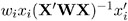L95M= name

• specifies a variable to contain the lower bound of an approximate 95% confidence interval for the expected value (mean). See also the description for the U95M= option, which follows.

L95= name

• specifies a variable to contain the lower bound of an approximate 95% confidence interval for an individual prediction. This includes the variance of the error as well as the variance of the parameter estimates. See also the description for the U95= option, which follows.

PARMS= names

• specifies variables in the output data set to contain parameter estimates. These can be the same variable names as listed in the PARAMETERS statement; however, you can choose new names for the parameters identified in the sequence from the parameter estimates table. A note log indicates which variable in the output data set is associated with each parameter name. Note that, for each of these new variables, the values are the same for every observation in the new data set.

PREDICTED= name

P= name

• specifies a variable in the output data set to contain the predicted values of the dependent variable.

RESIDUAL= name

R= name

• specifies a variable in the output data set to contain the residuals (actual values minus predicted values).

SSE= name

ESS= name

• specifies a variable to include in the new data set. The values for the variable are the residual sums of squares finally determined by the procedure. The values of the variable are the same for every observation in the new data set.

STDI= name

• specifies a variable to contain the standard error of the individual predicted value.

STDP= name

• specifies a variable to contain the standard error of the mean predicted value.

STDR= name

• specifies a variable to contain the standard error of the residual.

STUDENT= name

• specifies a variable to contain the studentized residuals, which are residuals divided by their standard errors.

U95M= name

• specifies a variable to contain the upper bound of an approximate 95% confidence interval for the expected value (mean). See also the description for the L95M= option.

U95= name

• specifies a variable to contain the upper bound of an approximate 95% confidence interval for an individual prediction. See also the description for the L95= option.

WEIGHT= name

• specifies a variable in the output data set that contains values of the special variable _WEIGHT_ .

PARAMETERS Statement

• PARAMETERS parameter=values ... ;

• PARMS parameter=values ... ;

A PARAMETERS (or PARMS) statement must come before the RUN statement. Several parameter names and values can appear. The parameter names must all be valid SAS names and must not duplicate the names of any variables in the data set to which the NLIN procedure is applied. Any parameters specified but not used in the MODEL statement are dropped from the estimation.

In each parameter=values specification, the parameter name identifies a parameter to be estimated, both in subsequent procedure statements and in the output. Values specify the possible starting values of the parameter.

Usually, only one value is specified for each parameter. If you specify several values for each parameter, PROC NLIN evaluates the model at each point on the grid. The value specifications can take any of several forms:

m	a single value
m 1, m 2, ... , mn	several values
m TO n	a sequence where m equals the starting value, n equals the ending value, and the increment equals 1
m TO n BY i	a sequence where m equals the starting value, n equals the ending value, and the increment is i
m 1, m 2 TO m 3	mixed values and sequences

This PARMS statement specifies five parameters and sets their possible starting values as shown:

  parms b0=0   b1=4 to 8   b2=0 to .6 by .2   b3=1, 10, 100   b4=0, .5, 1 to 4;  

Possible starting values
B0	B1	B2	B3	B4
	4	0.0	1	0.0
	5	0.2	10	0.5
	6	0.4	100	1.0
	7	0.6		2.0
	8			3.0
				4.0

Residual sums of squares are calculated for each of the 1 — 5 — 4 — 3 — 6 = 360 combinations of possible starting values. (This can take a long time.) See the Special Variables section beginning on page 3020 for information on programming parameter starting values.

RETAIN Statement

• RETAIN variable < =values >< ... variable < =values >> ;

The RETAIN statement declares retained variables and specifies their values. A retained variable is like a control variable (see the section CONTROL Statement on page 3011) except that it is retained only within iterations. An iteration involves a single pass through the data set.

Other Program Statements with PROC NLIN

PROC NLIN supports many statements that are similar to SAS programming statements used in a DATA step. However, there are some differences in capabilities; for additional information, see the section Incompatibilities with 6.11 and Earlier Versions of PROC NLIN beginning on page 3031.

Several SAS program statements can be used after the PROC NLIN statement. These statements can appear anywhere in the PROC NLIN statement, but new variables must be created before they appear in other statements. For example, the following statements are valid since they create the variable temp before they use it in the MODEL statement:

  proc nlin;   parms b0=0 to 2 by 0.5 b1=0.01 to 0.09 by 0.01;   temp=exp(-b1*x);   model y=b0*(1-temp);  

The following statements result in missing values for y because the variable temp is undefined before it is used:

  proc nlin;   parms b0=0 to 2 by 0.5 b1=0.01 to 0.09 by 0.01;   model y=b0*(1-temp);   temp=exp(-b1*x);  

PROC NLIN can process assignment statements, explicitly or implicitly subscripted ARRAY statements, explicitly or implicitly subscripted array references, IF statements, SAS functions, and program control statements. You can use program statements to create new SAS variables for the duration of the procedure. These variables are not permanently included in the data set to which PROC NLIN is applied. Program statements can include variables in the DATA= data set, parameter names, variables created by preceding program statements within PROC NLIN, and special variables used by PROC NLIN. All of the following SAS program statements can be used in PROC NLIN:

• ARRAY

• assignment ( y = a*x + b; )

• CALL

• DO

• iterative DO

• DO UNTIL

• DO WHILE

• END

• FILE

• GO TO

• IF-THEN/ELSE

• LINK-RETURN

• PUT (defaults to the list)

• RETURN

• SELECT

• sum ( y + 1; )

These statements can use the special variables created by PROC NLIN. Consult the section Special Variables beginning on page 3020 for more information on special variables.