Details

Theoretical Semivariogram Models

PROC VARIOGRAM computes the sample, or experimental semivariogram. Prediction of the spatial process at unsampled locations by techniques such as ordinary kriging requires a theoretical semivariogram or covariance.

When you use PROC VARIOGRAM and PROC KRIGE2D to perform spatial prediction, you must determine a suitable theoretical semivariogram based on the sample semivariogram. While there are various methods of fitting semivariogram models, such as least squares, maximum likelihood , and robust methods (Cressie 1993, section 2.6), these techniques are not appropriate for data sets resulting in a small number of variogram points. Instead, a visual fit of the variogram points to a few standard models is often satisfactory. Even when there are sufficient variogram points, a visual check against a fitted theoretical model is appropriate (Hohn 1988, p. 25ff).

In some cases, a plot of the experimental semivariogram suggests that a single theoretical model is inadequate. Nested models, anisotropic models, and the nugget effect increase the scope of theoretical models available. All of these concepts are discussed in this section. The specificationofthefinal theoretical model is provided by the syntax of PROC KRIGE2D.

Note the general flow of investigation. After a suitable choice is made of the LAGDIST= and MAXLAG= options and, possibly, the NDIR= option (or a DIRECTIONS statement), the experimental semivariogram is computed. Potential theoretical models, possibly incorporating nesting, anisotropy, and the nugget effect, are computed by a DATA step, then they are plotted against the experimental semivariogram and evaluated. A suitable theoretical model is thus found visually, and the specification of the model is used in PROC KRIGE2D. This flow is illustrated in Figure 37.3; also see the Getting Started section on page 4852 in the chapter on the VARIOGRAM procedure for an illustration in a simple case.

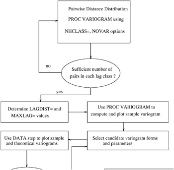
Figure 37.3: Flowchart for Variogram Selection

Four theoretical models are supported by PROC KRIGE2D: the spherical, Gaussian, exponential, and power models. For the first three types, the parameters a and c , corresponding to the RANGE= and SCALE= options in the MODEL statement in PROC KRIGE2D, have the same dimensions and have similar affects on the shape of ³ _z ( h ), as illustrated in the following paragraph.

In particular, the dimension of c is the same as the dimension of the variance of the spatial process { Z ( r ) , r ˆˆ D ‚ R ² }. The dimension of a is length with the same units as h.

These three model forms are now examined in more detail.

The Spherical Semivariogram Model

The form of the spherical model is

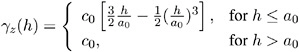
The shape is displayed in Figure 37.4 using range a = 1 and scale c = 4.

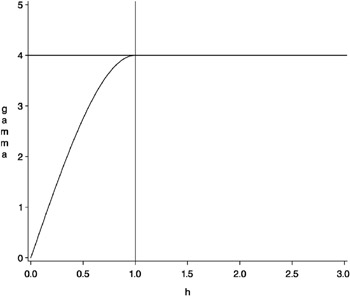
Figure 37.4: Spherical Semivariogram Model with Parameters a = 1 and c = 4

The vertical line at h = 1 is the effective range as defined by Duetsch and Journel (1992), or the range ˆˆ defined by Christakos (1992). This quantity, denoted r _ˆˆ , is the h -value where the covariance is approximately zero. For the spherical model, it is exactly zero; for the Gaussian and exponential models, the definition of r _ˆˆ is modified slightly.

The horizontal line at 4.0 variance units (corresponding to c = 4) is called the sill. In the case of the spherical model, ³ _z ( h ) actually reaches this value. For the other two model forms, the sill is a horizontal asymptote.

The Gaussian Semivariogram Model

The form of the Gaussian model is

The shape is displayed in Figure 37.5 using range a = 1 and scale c = 4.

Figure 37.5: Gaussian Semivariogram Model with Parameters a = 1 and c = 4

The vertical line at is the effective range, or the range ˆˆ (that is, the h -value where the covariance is approximately 5% of its value at zero).

The horizontal line at 4.0 variance units (corresponding to c = 4) is the sill; ³ _z ( h ) approaches the sill asymptotically.

The Exponential Semivariogram Model

The form of the exponential model is

The shape is displayed in Figure 37.6 using range a = 1and scale c = 4.

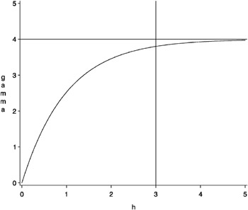
Figure 37.6: Exponential Semivariogram Model with Parameters a = 1 and c = 4

The vertical line at h = r _ˆˆ = 3 is the effective range, or the range ˆˆ (that is, the h -value where the covariance is approximately 5% of its value at zero).

The horizontal line at 4.0 variance units (corresponding to c =4) is the sill, as in the other model forms.

It is noted from Figure 37.5 and Figure 37.6 that the major distinguishing feature of the Gaussian and exponential forms is the shape in the neighborhood of the origin h =0. In general, small lags are important in determining an appropriate theoretical form based on a sample semivariogram.

The Power Semivariogram Model

The form of the power model is

For this model, the parameter a is a dimensionless quantity, with typical values 0 < a < 2. Note that the value of a = 1 yields a straight line. The parameter c has dimensions of the variance, as in the other models. There is no sill for the power model. The shape of the power model with a = 0 . 4 and c = 4 is displayed in Figure 37.7.

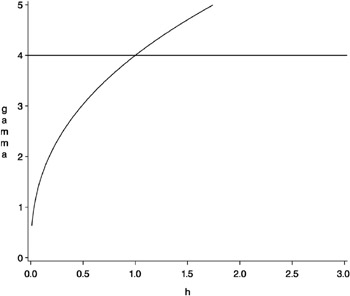
Figure 37.7: Power Semivariogram Model with Parameters a = 0 . 4 and c = 4

Nested Models

For a given set of spatial data, a plot of an experimental semivariogram may not seem to fit any one of the theoretical models. In such a case, the covariance structure of the spatial process may be a sum of two or more covariances. This is common in geologic applications where there are correlations at different length scales . At small lag distances h , the smaller scale correlations dominate, while the large scale correlations dominate at larger lag distances.

As an illustration, consider two semivariogram models, an exponential and a spherical.

and

with c _0,1 = 1 , a _0,1 = 2 . 5, c _0,2 = 2, and a _0,2 = 1. If both of these correlation structures are present in a spatial process { Z ( r ), r ˆˆ D }, then a plot of the experimental semivariogram would resemble the sum of these two semivariograms. This is illustrated in Figure 37.8.

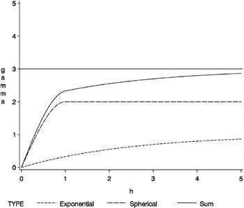
Figure 37.8: Sum of Exponential and Spherical Structures at Different Scales

This sum of ³ ₁ ( h ) and ³ ₂ ( h ) in Figure 37.8 does not resemble any single theoretical semivariogram; however, the shape at h = 1 is similar to a spherical. The asymptotic approach to a sill at three variance units, along with the shape around h = 0, indicates an exponential structure. Note that the sill value is the sum of the individual sills c _{, 1} = 1 and c _{, 2} = 2.

Refer to Hohn (1988, p. 38ff) for further examples of nested correlation structures.

The Nugget Effect

For all the variogram models considered previously, the following property holds:

However, a plot of the experimental semivariogram may indicate a discontinuity at h = 0; that is, ³ _z ( h ) ’ c _n > 0 as h ’ 0, while ³ _z (0) = 0. The quantity c _n is called the nugget effect ; this term is from mining geostatistics where nuggets literally exist, and it represents variations at a much smaller scale than any of the measured pairwise distances, that is, at distances h << h _min, where

There are conceptual and theoretical difficulties associated with a nonzero nugget effect; refer to Cressie (1993, section 2.3.1) and Christakos (1992, section 7.4.3) for details. There is no practical difficulty however; you simply visually extrapolate the experimental semivariogram as h ’ 0. The importance of availability of data at small lag distances is again illustrated.

As an example, an exponential semivariogram with a nugget effect c _n has the form

and

This is illustrated in Figure 37.9 for parameters a = 1, c = 4, and nugget effect c _n = 1 . 5.

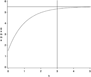
Figure 37.9: Exponential Semivariogram Model with a Nugget Effect c _n = 1 . 5

You can specify the nugget effect in PROC KRIGE2D with the NUGGET= option in the MODEL statement. It is a separate, additive term independent of direction; that is, it is isotropic. There is a way to approximate an anisotropic nugget effect; this is described in the following section.

Anisotropic Models

In all the theoretical models considered previously, the lag distance h entered as a scalar value. This implies that the correlation between the spatial process at two point pairs P ₁ , P ₂ is dependent only on the separation distance h = P ₁ P ₂ , not on the orientation of the two points. A spatial process { Z ( r ), r ˆˆ D } with this property is called isotropic, as is the associated covariance or semivariogram.

However, real spatial phenomena often show directional effects. Particularly in geologic applications, measurements along a particular direction may be highly correlated, while the perpendicular direction shows little or no correlation. Such processes are called anisotropic. Refer to Journel and Huijbregts (1978, section III.B.4) for more details.

There are two types of anisotropy. The simplest type occurs when the same covariance form and scale parameter c is present in all directions but the range a changes with direction. In this case, there is a single sill, but the semivariogram reaches the sill in a shorter lag distance along a certain direction.

This type of anisotropy is called geometric and is discussed in the following section.

Geometric Anisotropy

Geometric anisotropy is illustrated in Figure 37.10, where an anisotropic Gaussian semivariogram is plotted. The two curves displayed in this figure are generated using a = 1 in the NE “SW direction and a = 3 in the SE “NW direction.

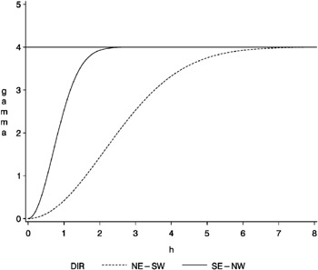
Figure 37.10: Geometric Anisotropy with Major Axis along E “W Direction

As you can see from the figure, the SE “NW curve gets close to the sill at approximately h = 2, while the NE “SW curve does so at h = 6. The ratio of the shorter to longer distance is . This is the value to use in the RATIO= parameter in the MODEL statement in PROC KRIGE2D. Since the longer, or major, axis is in the NE_SW direction, the ANGLE= parameter in the MODEL statement in PROC KRIGE2D should be 45 ° (all angles are measured clockwise from north).

The terminology associated with geometric anisotropy is that of ellipses. To see how this comes about, consider the following hypothetical set of calculations.

Let { Z ( r ), r ˆˆ D } be a geometrically anisotropic process, and assume that there are sufficient data points to calculate an experimental semivariogram at a large number of angle classes ˆˆ { 0 , , 2 , , 180 ° }. At each of these angles , the experimental semivariogram is plotted and the effective range r _ˆˆ is recorded. A diagram, in polar coordinates, of ( r _ˆˆ , ) yields an ellipse, with the major axis in the direction of the largest r _ˆˆ and the minor axis perpendicular. Denote the largest r _ˆˆ by , the smallest by , and their ratio by

By a rotation, a new set of axes are aligned along the major and minor axis. Then, a rescaling elongates the minor axis so its length equals that of the major axis of the ellipse.

First, the angle of the major axis of the ellipse (measured clockwise from north) is transformed to standard Cartesian orientation or counter-clockwise from the x-axis (east). Let • = 90 ° ˆ’ denote the transformed angle. The matrix to transform the distance h is in terms of • and the ratio R and it is given by

For a given point pair P ₁ P ₂ , with coordinates ( x ₁ ,y ₁ ) , ( x ₂ ,y ₂ ), the transformed interpair distance is computed by first transforming the components x = x ₁ ˆ’ x ₂ and y = y ₁ ˆ’ y ₂ by

The transformed interpair distance is then

The original semivariogram, a function of both h and , is then transformed to a function only of h ² :

This single semivariogram is then used for kriging purposes.

The interpretation of the major/minor axis in the case of geometric anisotropy is that the direction of the major axis is the direction in which the spatial process { Z ( r ), r ˆˆ D } is most highly correlated; the process is least correlated in the perpendicular direction.

In some cases, these directions are known a priori . This can occur in mining applications where the geology of a region is known in advance. In most cases, however, nothing is known about possible anisotropy. Depending on the amount of data available, using four to six directions is usually sufficient to determine the presence of anisotropy and find the approximate major/minor axis directions.

The most convenient way of performing this is to use the NDIR= option in the COMPUTE statement in PROC VARIOGRAM to obtain a separate experimental semivariogram for each direction. After determining the direction of the major axis, use a DIRECTIONS statement on a subsequent run of PROC VARIOGRAM with this direction and its perpendicular direction. For example, if the initial run of PROC VARIOGRAM with NDIR=6 in the COMPUTE statement indicates that = 45 ° is the major axis (has the largest r _ˆˆ ), then rerun PROC VARIOGRAM with

  DIRECTIONS 45,135;  

Then, determine the ratio of r _ˆˆ for the minor and major axis for the RATIO= parameter in the COMPUTE statement of PROC KRIGE2D. This ratio is ‰ 1 for modeling geometric anisotropy. In the other type of anisotropy, zonal anisotropy, the RATIO= parameter is set to a large number for reasons explained in the following section.

Zonal Anisotropy

In zonal anisotropy, either the form covariance structure or the parameter c (or both) is different in different directions. In particular, the sill is different for different directions. In geologic applications, this is the more common type of anisotropy. It is not possible to transform such a structure into an isotropic semivariogram.

Instead, nesting and geometric anisotropy are used together to approximate zonal anisotropy. For example, suppose the spatial process has a correlation structure in the N “S direction described by ³ _{z, 1} , a spherical model with sill at c = 6 and range a = 2, while in the E “W direction the correlation structure, described by ³ _{z, 2} , is again a spherical model but with sill at c = 3 and range a = 1.

You can approximate this structure in PROC KRIGE2D by specifying two nested models with large RATIO= values. In particular, the appropriate MODEL statement is

  MODEL FORM=(S,S) ANGLE=(0,90) SCALE=(6,3)   RANGE=(2,1) RATIO=(1E8,1E8);  

The large values of the RATIO= parameter for each nested structure have the effect of an infinite range parameter in the direction of the minor axis. Hence, there is no variation in ³ _{z, 1} in the E “W direction and no variation in ³ _{z, 2} in the N “S direction.

Anisotropic Nugget Effect

Note that an isotropic nugget effect can be approximated by using nested models, with one of the nested models having a small range. Applying a geometric anisotropy specification to this nested structure results in an anisotropic nugget effect.

Details of Ordinary Kriging

Introduction

There are three common characteristics often observed with spatial data (that is, data indexed by their spatial locations).

1. slowly varying, large-scale variations in the measured values

2. irregular, small-scale variations

3. similarity of measurements at locations close together

As an illustration, consider a hypothetical example in which an organic solvent leaks from an industrial site and spreads over a large area. Assume the solvent is absorbed and immobilized into the subsoil above any ground-water level, so you can ignore any time dependence.

For you to find the areal extent and the concentration values of the solvent, measurements are required. Although the problem is inherently three-dimensional, if you measure total concentration in a column of soil or take a depth-averaged concentration, it can be handled reasonably well with two-dimensional techniques.

You usually assume that measured concentrations are higher closer to the source and decrease at larger distances from the source. On top of this smooth variation, there are small-scale variations in the measured concentrations, due perhaps to the inherent variability of soil properties.

You also tend to suspect that measurements made close together yield similar concentration values, while measurements made far apart can have very different values.

These physically reasonable qualitative statements have no explicit probabilistic content, and there are a number of numerical smoothing techniques, such as inverse distance weighting and splines, that make use of large-scale variations and close distance-close value characteristics of spatial data to interpolate the measured concentrations for contouring purposes.

While characteristics (i) and (iii) are handled by such smoothing methods, characteristic (ii), the small-scale residual variation in the concentration field, is not accounted for.

There may be situations, due to the use of the prediction map or due to the relative magnitude of the irregular fluctuations, where you cannot ignore these small-scale irregular fluctuations. In other words, the smoothed or estimated values of the concentration field alone are not a sufficient characterization; you also need the possible spread around these contoured values.

Spatial Random Fields

One method of incorporating characteristic (ii) into the construction of a contour map is to model the concentration field as a spatial random field (SRF). The mathematical details of SRF models are given in a number of texts , for example, Cressie (1993) and Christakos (1992). The mathematics of SRFs are formidable. However, under certain simplifying assumptions, they produce classical linear estimators with very simple properties, allowing easy implementation for prediction purposes. These estimators, primarily ordinary kriging (OK), give both a prediction and a standard error of prediction at unsampled locations. This allows the construction of a map of both predicted values and level of uncertainty about the predicted values.

The key assumption in applying the SRF formalism is that the measurements come from a single realization of the SRF. However, in most geostatistical applications, the focus is on a single, unique realization. This is unlike most other situations in stochastic modeling in which there will be future experiments or observational activities (at least conceptually) under similar circumstances. This renders many traditional ideas of statistical inference ambiguous and somewhat counterintuitive.

There are additional logical and methodological problems in applying a stochastic model to a unique but partly unknown natural process; refer to the introduction in Matheron (1971) and Cressie (1993, section 2.3). These difficulties have resulted in attempts to frame the estimation problem in a completely deterministic way (Isaaks and Srivastava 1988; Journel 1985).

Additional problems with kriging, and with spatial estimation methods in general, are related to the necessary assumption of ergodicity of the spatial process. This assumption is required to estimate the covariance or semivariogram from sample data. Details are provided in Cressie (1993, pp. 52 “58).

Despite these difficulties, ordinary kriging remains a popular and widely used tool in modeling spatial data, especially in generating surface plots and contour maps. An abbreviated derivation of the OK estimator for point estimation and the associated standard error is discussed in the following section. Full details are given in Journel and Huijbregts (1978), Christakos (1992), and Cressie (1993).

Ordinary Kriging

Denote the SRF by Z ( r ), r ˆˆ D ‚ R ² . Following the notation in Cressie (1993), the following model for Z ( r ) is assumed:

Here, ¼ is the fixed, unknown mean of the process, and µ ( r ) is a zero mean SRF representing the variation around the mean.

In most practical applications, an additional assumption is required in order to estimate the covariance C _z of the Z ( r ) process. This assumption is second-order stationarity:

This requirement can be relaxed slightly when you are using the semivariogram instead of the covariance. In this case, second-order stationarity is required of the differences µ ( r ₁ ) ˆ’ µ ( r ₂ ) rather than µ ( r ):

By performing local kriging, the spatial processes represented by the previous equation for Z( r ) are more general than they appear. In local kriging, at an unsampled location r , a separate model is fit using only data in a neighborhood of r .Thishas the effect of fitting a separate mean ¼ at each point, and it is similar to the kriging with trend (KT) method discussed in Journel and Rossi (1989).

Given the N measurements Z ( r ₁ ) , ,Z ( r _N ) at known locations r ₁ , ,r _N , you want to obtain an estimate of Z at an unsampled location r . When the following three requirements are imposed on the estimator , the OK estimator is obtained.

1. is linear in Z ( r ₁ ) , · · ·,Z ( r _N ).

2. is unbiased .

3. minimizes the mean-square prediction error E ( Z (r ) “ (r )) ² .

Linearity requires the following form for (r ):

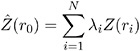
Applying the unbiasedness condition to the preceding equation yields

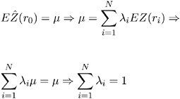
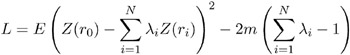
Finally, the third condition requires a constrained linear optimization involving » ₁ , · · ·, » _N and a Lagrange parameter 2 m . This constrained linear optimization can be expressed in terms of the function L ( » ₁ , · · ·, » _N , m ) given by

Define the N — 1 column vector » by

and the ( N + 1) — 1 column vector » by

The optimization is performed by solving

in terms of » ₁ , · · ·, » _N and m .

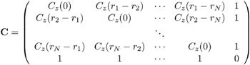
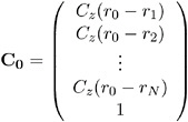
The resulting matrix equation can be expressed in terms of either the covariance C _z ( r ) or semivariogram ³ _z ( r ). In terms of the covariance, the preceding equation results in the following matrix equation:

where

and

The solution to the previous matrix equation is

Using this solution for » and m , the ordinary kriging estimate at r is

with associated prediction error

where c is C with the 1 in the last row removed, making it an N — 1 vector.

These formulas are used in the best linear unbiased prediction (BLUP) of random variables (Robinson 1991). Further details are provided in Cressie (1993, pp. 119 “123).

Because of possible numeric problems when solving the previous matrix equation, Duetsch and Journel (1992) suggest replacing the last row and column of 1sinthe preceding matrix C by C _z (0), keeping the 0 in the ( N + 1 , N + 1) position and similarly replacing the last element in the preceding right-hand vector C with C _z (0). This results in an equivalent system but avoids numeric problems when C _z (0) is large or small relative to 1.

Output Data Sets

The KRIGE2D procedure produces two data sets: the OUTEST= SAS-data-set and the OUTNBHD= SAS-data-set . These data sets are described as follows .

OUTEST=SAS-data-set

The OUTEST= data set contains the kriging estimates and the associated standard errors. The OUTEST= data set contains the following variables:

• ESTIMATE , which is the kriging estimate for the current variable

• GXC , which is the x-coordinate of the grid point at which the kriging estimate is made

• GYC , which is the y-coordinate of the grid point at which the kriging estimate is made

• LABEL , which is the label for the current PREDICT/MODEL combination producing the kriging estimate. If you do not specify a label, default labels of the form Pred j .Model k are used.

• NPOINTS , which is the number of points used in the estimation. This number varies for each grid point if local kriging is performed.

• STDERR , which is the standard error of the kriging estimate

• VARNAME , which is the variable name

OUTNBHD=SAS-data-set

When you specify the RADIUS= option or the NUMPOINTS= option in the PREDICT statement, local kriging is performed. Local kriging is simply ordinary kriging at a given grid location using only those data points in a neighborhood defined by the RADIUS= value or the NUMPOINTS= value.

The OUTNBHD= data set contains one observation for each data point in each neighborhood. Hence, this data set can be large. For example, if the grid specification results in 1,000 grid points and each grid point has a neighborhood of 100 points, the resulting OUTNBHD= data set contains 100,000 points.

The OUTNBHD= data set contains the following variables:

• GXC , which is the x-coordinate of the grid point

• GYC , which is the y-coordinate of the grid point

• LABEL , which is the label for the current PREDICT/MODEL combination. If you do not specify a label, default labels of the form Pred j .Model k are used.

• NPOINTS , which is the number of points used in the estimation

• RADIUS , which is the radius used for each neighborhood

• VALUE , which is the value of the variable at the current data point

• VARNAME , which is the variable name of the current variable

• XC , which is the x-coordinate of the current data point

• YC , which is the y-coordinate of the current data point

Computational Resources

To generate a predicted value at a single grid point using N data points, PROC KRIGE2D must solve the following kriging system:

where C is ( N + 1) — ( N + 1), and the right-hand side vector C is ( N +1) — 1.

Holding the matrix and vector associated with this system in core requires approximately doubles (with typically eight bytes per double). The CPU time used in solving the system is proportional to N ³ . For large N , this time dominates the time to compute the elements of the covariance matrix C from the specified covariance or variogram model. This latter computation is proportional to N ² .

For local kriging, the kriging system is set up and solved for each grid point. Part of the set up process involves determining the neighborhood of each grid point. A fast K-D tree algorithm is used to determine neighborhoods. For G grid points, the dominant CPU time factor is setting up and solving the G kriging systems. The N in the preceding algorithm is the number of data points in a given neighborhood, and it can differ for each grid point.

In global kriging, the entire input data set and all grid points are used to set up and solve the single system

Again C is ( N + 1) — ( N + 1), but » is now ( N + 1) — G , where G is the number of grid points, and N is the number of nonmissing observations in the input data set. The right-hand side matrix C is ( N +1) — G . Memory requirements are approximately doubles. The CPU time used in solving the system is still dominated by the N ³ factorization of the left-hand side.