Details
Generalized Linear Models Theory
This is a brief introduction to the theory of generalized linear models. See the References section on page 1728 for sources of more detailed information.
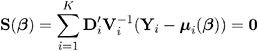
Response Probability Distributions
In generalized linear models, the response is assumed to possess a probability distribution of the exponential form. That is, the probability density of the response Y for continuous response variables , or the probability function for discrete responses, can be expressed as
for some functions a , b , and c that determine the specific distribution. For fixed ![]() , this is a one parameter exponential family of distributions. The functions a and c are such that a (
, this is a one parameter exponential family of distributions. The functions a and c are such that a ( ![]() ) =
) = ![]() /w and c = c ( y,
/w and c = c ( y, ![]() /w ), where w is a known weight for each observation. A variable representing w in the input data set may be specified in the WEIGHT statement. If no WEIGHT statement is specified, w i = 1 for all observations.
/w ), where w is a known weight for each observation. A variable representing w in the input data set may be specified in the WEIGHT statement. If no WEIGHT statement is specified, w i = 1 for all observations.
Standard theory for this type of distribution gives expressions for the mean and variance of Y .
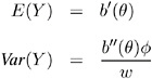
where the primes denote derivatives with respect to . If ¼ represents the mean of Y, then the variance expressed as a function of the mean is
where V is the variance function .
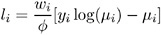
Probability distributions of the response Y in generalized linear models are usually parameterized in terms of the mean ¼ and dispersion parameter ![]() instead of the natural parameter . The probability distributions that are available in the GENMOD procedure are shown in the following list. The PROC GENMOD scale parameter and the variance of Y are also shown.
instead of the natural parameter . The probability distributions that are available in the GENMOD procedure are shown in the following list. The PROC GENMOD scale parameter and the variance of Y are also shown.
-
Normal:
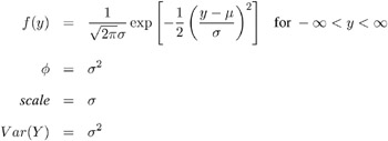
-
Inverse Gaussian:
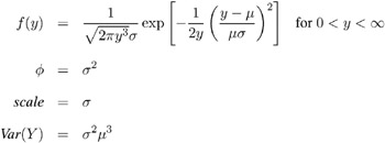
-
Gamma:
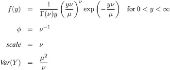
-
Negative Binomial:
-
Poisson:
-
Binomial:
-
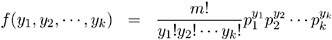
Multinomial:
The negative binomial distribution contains a parameter k , called the negative binomial dispersion parameter. This is not the same as the generalized linear model dispersion ![]() , but it is an additional distribution parameter that must be estimated or set to a fixed value.
, but it is an additional distribution parameter that must be estimated or set to a fixed value.
For the binomial distribution, the response is the binomial proportion Y = events/trials . The variance function is V ( ¼ ) = ¼ (1 ˆ’ ¼ ), and the binomial trials parameter n is regarded as a weight w .
If a weight variable is present, ![]() is replaced with
is replaced with ![]() /w , where w is the weight variable.
/w , where w is the weight variable.
PROC GENMOD works with a scale parameter that is related to the exponential family dispersion parameter ![]() instead of with
instead of with ![]() itself. The scale parameters are related to the dispersion parameter as shown previously with the probability distribution definitions. Thus, the scale parameter output in the Analysis of Parameter Estimates table is related to the exponential family dispersion parameter. If you specify a constant scale parameter with the SCALE= option in the MODEL statement, it is also related to the exponential family dispersion parameter in the same way.
itself. The scale parameters are related to the dispersion parameter as shown previously with the probability distribution definitions. Thus, the scale parameter output in the Analysis of Parameter Estimates table is related to the exponential family dispersion parameter. If you specify a constant scale parameter with the SCALE= option in the MODEL statement, it is also related to the exponential family dispersion parameter in the same way.
Link Function
The mean ¼ i of the response in the i th observation is related to a linear predictor through a monotonic differentiable link function g .
Here, x i is a fixed known vector of explanatory variables, and ² is a vector of unknown parameters.
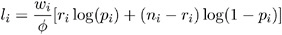
Log- Likelihood Functions
Log-likelihood functions for the distributions that are available in the procedure are parameterized in terms of the means ¼ i and the dispersion parameter ![]() . The term y i represents the response for the i th observation, and w i represents the known dispersion weight. The log-likelihood functions are of the form
. The term y i represents the response for the i th observation, and w i represents the known dispersion weight. The log-likelihood functions are of the form
where the sum is over the observations. The forms of the individual contributions
are shown in the following list; the parameterizations are expressed in terms of the mean and dispersion parameters.
-
Normal:
-
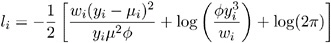
Inverse Gaussian:
-
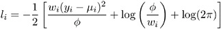
Gamma:
-
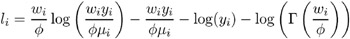
Negative Binomial:

-
Poisson:
-
Binomial:
-
Multinomial:
For the binomial, multinomial, and Poisson distribution, terms involving binomial coefficients or factorials of the observed counts are dropped from the computation of the log-likelihood function since they do not affect parameter estimates or their estimated covariances. The value of ![]() used in computing the reported log-likelihood is either the final estimated value, or the fixed value, if the dispersion parameter is fixed.
used in computing the reported log-likelihood is either the final estimated value, or the fixed value, if the dispersion parameter is fixed.
Maximum Likelihood Fitting
The GENMOD procedure uses a ridge-stabilized Newton-Raphson algorithm to maximize the log-likelihood function L ( y , ¼ , ![]() ) with respect to the regression parameters. By default, the procedure also produces maximum likelihood estimates of the scale parameter as definedinthe Response Probability Distributions section (page 1650) for the normal, inverse Gaussian, negative binomial, and gamma distributions.
) with respect to the regression parameters. By default, the procedure also produces maximum likelihood estimates of the scale parameter as definedinthe Response Probability Distributions section (page 1650) for the normal, inverse Gaussian, negative binomial, and gamma distributions.
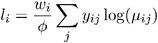
On the r th iteration, the algorithm updates the parameter vector ² r with
where H is the Hessian (second derivative) matrix, and s is the gradient (first derivative) vector of the log-likelihood function, both evaluated at the current value of the parameter vector. That is,
and
In some cases, the scale parameter is estimated by maximum likelihood. In these cases, elements corresponding to the scale parameter are computed and included in s and H .
If · i = x i ² ² is the linear predictor for observation i and g is the link function, then · i = g ( ¼ i ), so that ¼ i = g ˆ’ 1 ( x i ² ² ) is an estimate of the mean of the i th observation, obtained from an estimate of the parameter vector ² .
The gradient vector and Hessian matrix for the regression parameters are given by
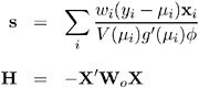
where X is the design matrix, x i is the transpose of the i th row of X , and V is the variance function. The matrix W o is diagonal with its i th diagonal element
where
The primes denote derivatives of g and V with respect to ¼ . The negative of H is called the observed information matrix. The expected value of W o is a diagonal matrix W e with diagonal values w ei . If you replace W o with W e , then the negative of H is called the expected information matrix. W e is the weight matrix for the Fishers scoring method of fitting. Either W o or W e can be used in the update equation. The GENMOD procedure uses Fishers scoring for iterations up to the number specified by the SCORING option in the MODEL statement, and it uses the observed information matrix on additional iterations.
Covariance and Correlation Matrix
The estimated covariance matrix of the parameter estimator is given by
where H is the Hessian matrix evaluated using the parameter estimates on the last iteration. Note that the dispersion parameter, whether estimated or specified, is incorporated into H . Rows and columns corresponding to aliased parameters are not included in & pound ; .
The correlation matrix is the normalized covariance matrix. That is, if ƒ ij is an element of , then the corresponding element of the correlation matrix is ƒ ij / ƒ i ƒ j , where ![]() .
.
Goodness of Fit
Two statistics that are helpful in assessing the goodness of fit of a given generalized linear model are the scaled deviance and Pearsons chi-square statistic. For a fixed value of the dispersion parameter ![]() , the scaled deviance is defined to be twice the difference between the maximum achievable log likelihood and the log likelihood at the maximum likelihood estimates of the regression parameters.
, the scaled deviance is defined to be twice the difference between the maximum achievable log likelihood and the log likelihood at the maximum likelihood estimates of the regression parameters.
Note that these statistics are not valid for GEE models.
If l ( y , ¼ ) is the log-likelihood function expressed as a function of the predicted mean values ¼ and the vector y of response values, then the scaled deviance is defined by
For specific distributions, this can be expressed as
where D is the deviance. The following table displays the deviance for each of the probability distributions available in PROC GENMOD.
| Distribution | Deviance |
|---|---|
| normal | |
| Poisson | |
| binomial | |
| gamma | |
| inverse Gaussian | |
| multinomial | |
| negative binomial | |
In the binomial case, y i = r i /m i , where r i is a binomial count and m i is the binomial number of trials parameter.
In the multinomial case, y ij refers to the observed number of occurrences of the j th category for the i th subpopulation defined by the AGGREGATE= variable, m i is the total number in the i th subpopulation, and p ij is the category probability.
Pearsons chi-square statistic is defined as
and the scaled Pearsons chi-square is X 2 / ![]() .
.
The scaled version of both of these statistics, under certain regularity conditions, has a limiting chi-square distribution, with degrees of freedom equal to the number of observations minus the number of parameters estimated. The scaled version can be used as an approximate guide to the goodness of fit of a given model. Use caution before applying these statistics to ensure that all the conditions for the asymptotic distributions hold. McCullagh and Nelder (1989) advise that differences in deviances for nested models can be better approximated by chi-square distributions than the deviances themselves .
In cases where the dispersion parameter is not known, an estimate can be used to obtain an approximation to the scaled deviance and Pearsons chi-square statistic. One strategy is to fit a model that contains a sufficient number of parameters so that all systematic variation is removed, estimate ![]() from this model, and then use this estimate in computing the scaled deviance of sub-models. The deviance or Pearsons chi-square divided by its degrees of freedom is sometimes used as an estimate of the dispersion parameter
from this model, and then use this estimate in computing the scaled deviance of sub-models. The deviance or Pearsons chi-square divided by its degrees of freedom is sometimes used as an estimate of the dispersion parameter ![]() . For example, since the limiting chi-square distribution of the scaled deviance D * = D/
. For example, since the limiting chi-square distribution of the scaled deviance D * = D/ ![]() has n ˆ’ p degrees of freedom, where n is the number of observations and p the number of parameters, equating D * to its mean and solving for
has n ˆ’ p degrees of freedom, where n is the number of observations and p the number of parameters, equating D * to its mean and solving for ![]() yields
yields ![]() = D/ ( n ˆ’ p ). Similarly, an estimate of
= D/ ( n ˆ’ p ). Similarly, an estimate of ![]() based on Pearsons chi-square X 2 is
based on Pearsons chi-square X 2 is ![]() = X 2 / ( n ˆ’ p ). Alternatively, a maximum likelihood estimate of
= X 2 / ( n ˆ’ p ). Alternatively, a maximum likelihood estimate of ![]() can be computed by the procedure, if desired. See the discussion in the Type 1 Analysis section on page 1665 for more on the estimation of the dispersion parameter.
can be computed by the procedure, if desired. See the discussion in the Type 1 Analysis section on page 1665 for more on the estimation of the dispersion parameter.
Dispersion Parameter
There are several options available in PROC GENMOD for handling the exponential distribution dispersion parameter. The NOSCALE and SCALE options in the MODEL statement affect the way in which the dispersion parameter is treated. If you specify the SCALE=DEVIANCE option, the dispersion parameter is estimated by the deviance divided by its degrees of freedom. If you specify the SCALE=PEARSON option, the dispersion parameter is estimated by Pearsons chi-square statistic divided by its degrees of freedom.
Otherwise, values of the SCALE and NOSCALE options and the resultant actions are displayed in the following table.
| NOSCALE | SCALE= value | Action |
|---|---|---|
| present | present | scale fixed at value |
| present | not present | scale fixed at 1 |
| not present | not present | scale estimated by ML |
| not present | present | scale estimated by ML, starting point at value |
The meaning of the scale parameter displayed in the Analysis Of Parameter Estimates table is different for the Gamma distribution than for the other distributions. The relation of the scale parameter as used by PROC GENMOD to the exponential family dispersion parameter ![]() is displayed in the following table. For the binomial and Poisson distributions,
is displayed in the following table. For the binomial and Poisson distributions, ![]() is the overdispersion parameter, as defined in the Overdispersion section, which follows .
is the overdispersion parameter, as defined in the Overdispersion section, which follows .
| Distribution | Scale |
|---|---|
| normal | |
| inverse Gaussian | |
| gamma | |
| binomial | |
| Poisson | |
In the case of the negative binomial distribution, PROC GENMOD reports the dispersion parameter estimated by maximum likelihood. This is the negative binomial parameter k defined in the Response Probability Distributions section (page 1650).
Overdispersion
Overdispersion is a phenomenon that sometimes occurs in data that are modeled with the binomial or Poisson distributions. If the estimate of dispersion after fitting, as measured by the deviance or Pearsons chi-square, divided by the degrees of freedom, is not near 1, then the data may be overdispersed if the dispersion estimate is greater than 1 or underdispersed if the dispersion estimate is less than 1. A simple way to model this situation is to allow the variance functions of these distributions to have a multiplicative overdispersion factor ![]() .
.
-
binomial: V ( ¼ ) =
 ¼ (1 ˆ’ ¼ )
 -
Poisson: V ( ¼ ) =
¼
The models are fit in the usual way, and the parameter estimates are not affected by the value of ![]() . The covariance matrix, however, is multiplied by
. The covariance matrix, however, is multiplied by ![]() , and the scaled deviance and log likelihoods used in likelihood ratio tests are divided by
, and the scaled deviance and log likelihoods used in likelihood ratio tests are divided by ![]() . The profile likelihood function used in computing confidence intervals is also divided by
. The profile likelihood function used in computing confidence intervals is also divided by ![]() . If you specify an WEIGHT statement,
. If you specify an WEIGHT statement, ![]() is divided by the value of the WEIGHT variable for each observation. This has the effect of multiplying the contributions of the log-likelihood function, the gradient, and the Hessian by the value of the WEIGHT variable for each observation.
is divided by the value of the WEIGHT variable for each observation. This has the effect of multiplying the contributions of the log-likelihood function, the gradient, and the Hessian by the value of the WEIGHT variable for each observation.
The SCALE= option in the MODEL statement enables you to specify a value of ![]() for the binomial and Poisson distributions. If you specify the SCALE=DEVIANCE option in the MODEL statement, the procedure uses the deviance divided by degrees of freedom as an estimate of
for the binomial and Poisson distributions. If you specify the SCALE=DEVIANCE option in the MODEL statement, the procedure uses the deviance divided by degrees of freedom as an estimate of ![]() , and all statistics are adjusted appropriately. You can use Pearsons chi-square instead of the deviance by specifying the SCALE=PEARSON option.
, and all statistics are adjusted appropriately. You can use Pearsons chi-square instead of the deviance by specifying the SCALE=PEARSON option.
The function obtained by dividing a log-likelihood function for the binomial or Poisson distribution by a dispersion parameter is not a legitimate log-likelihood function. It is an example of a quasi-likelihood function. Most of the asymptotic theory for log likelihoods also applies to quasi-likelihoods, which justifies computing standard errors and likelihood ratio statistics using quasi-likelihoods instead of proper log likelihoods. Refer to McCullagh and Nelder (1989, Chapter 9) and McCullagh (1983) for details on quasi-likelihood functions.
Although the estimate of the dispersion parameter is often used to indicate overdispersion or underdispersion, this estimate may also indicate other problems such as an incorrectly specified model or outliers in the data. You should carefully assess whether this type of model is appropriate for your data.
Specification of Effects
Each term in a model is called an effect. Effects are specified in the MODEL statement in the same way as in the GLM procedure. You specify effects with a special notation that uses variable names and operators. There are two types of variables, classification (or class ) variables and continuous variables. There are two primary types of operators, crossing and nesting . A third type, the bar operator, is used to simplify effect specification. Crossing is the type of operator most commonly used in generalized linear models.
Variables that identify classification levels are called class variables in the SAS System and are identified in a CLASS statement. These may also be called categorical, qualitative, discrete, or nominal variables. Class variables can be either character or numeric. The values of class variables are called levels . For example, the class variable Sex could have levels ˜male and ˜ female .
In a model, an explanatory variable that is not declared in a CLASS statement is assumed to be continuous. Continuous variables must be numeric. For example, the heights and weights of subjects in an experiment are continuous variables.
The types of effects most useful in generalized linear models are shown in the following list. Assume that A , B , and C are class variables and that X1 and X2 are continuous variables.
-
Regressor effects are specified by writing continuous variables by themselves: X1 , X2 .
-
Polynomial effects are specified by joining two or more continuous variables with asterisks : X1 * X2 .
-
Main effects are specified by writing class variables by themselves: A , B , C .
-
Crossed effects (interactions) are specified by joining two or more class variables with asterisks: A * B , B * C , A * B * C .
-
Nested effects are specified by following a main effect or crossed effect with a class variable or list of class variables enclosed in parentheses: B ( A ), C ( B A ), A * B ( C ). In the preceding example, B ( A ) is B nested within A .
-
Combinations of continuous and class variables can be specified in the same way using the crossing and nesting operators.
The bar operator consists of two effects joined with a vertical bar (). It is shorthand notation for including the left-hand side, the right-hand side, and the cross between them as effects in the model. For example, A B is equivalent to A B A * B . The effects in the bar operator can be class variables, continuous variables, or combinations of effects defined using operators. Multiple bars are permitted. For example, A B C means A B C A*B A*C B*C A*B*C .
You can specify the maximum number of variables in any effect that results from bar evaluation by specifying the maximum number, preceded by an @ sign. For example, A B C @2 results in effects that involve two or fewer variables: A B C A*B A*C B*C .
For further information on types of effects and their specification, see Chapter 32, The GLM Procedure.
Parameterization Used in PROC GENMOD
Design Matrix
The linear predictor part of a generalized linear model is
where ² is an unknown parameter vector and X is a known design matrix. By default, all models automatically contain an intercept term; that is, the first column of X contains all 1s. Additional columns of X are generated for classification variables, regression variables, and any interaction terms included in the model. PROC GENMOD parameterizes main effects and interaction terms using the same ordering rules that PROC GLM uses. This is important to understand when you want to construct likelihood ratios for custom contrasts using the CONTRAST statement. See Chapter 32, The GLM Procedure, for more details on model parameterization.
Some columns of X can be linearly dependent on other columns due to specifying an overparameterized model. For example, when you specify a model consisting of an intercept term and a class variable, the column corresponding to any one of the levels of the class variable is linearly dependent on the other columns of X . PROC GENMOD handles this in the same manner as PROC GLM. The columns of X ² X are checked in the order in which the model is specified for dependence on preceding columns. If a dependency is found, the parameter corresponding to the dependent column is set to 0 along with its standard error to indicate that it is not estimated. The order in which the levels of a class variable are checked for dependencies can be set by the ORDER= option in the PROC GENMOD statement.
You can exclude the intercept term from the model by specifying the NOINT option in the MODEL statement.
Missing Level Combinations
All levels of interaction terms involving classification variables may not be represented in the data. In that case, PROC GENMOD does not include parameters in the model for the missing levels.
CLASS Variable Parameterization
Consider a model with one CLASS variable A with four levels, 1, 2, 5, and 7. Details of the possible choices for the PARAM= option follow.
| EFFECT | Three columns are created to indicate group membership of the nonreference levels. For the reference level, all three dummy variables have a value of ˆ’ 1. For instance, if the reference level is 7 (REF=7), the design matrix columns for A are as follows. | |||
| Effect Coding | ||||
| A | Design Matrix | |||
| A1 | A2 | A5 | ||
| 1 | 1 |
|
| |
| 2 |
| 1 |
| |
| 5 |
|
| 1 | |
| 7 | ˆ’ 1 | ˆ’ 1 | ˆ’ 1 | |
| Parameter estimates of CLASS main effects using the effect coding scheme estimate the difference in the effect of each nonreference level compared to the average effect over all four levels. | ||||
| GLM | As in PROC GLM, four columns are created to indicate group membership. The design matrix columns for A are as follows. | ||||
| GLM Coding | |||||
| A | Design Matrix | ||||
| A1 | A2 | A5 | A7 | ||
| 1 | 1 |
|
|
| |
| 2 |
| 1 |
|
| |
| 5 |
|
| 1 |
| |
| 7 |
|
|
| 1 | |
| Parameter estimates of CLASS main effects using the GLM coding scheme estimate the difference in the effects of each level compared to the last level. | |||||
| ORDINAL THERMOMETER | Three columns are created to indicate group membership of the higher levels of the effect. For the first level of the effect (which for A is 1), all three dummy variables have a value of 0. The design matrix columns for A are as follows. | ||||
| Ordinal Coding | |||||
| A | Design Matrix | ||||
| A2 | A5 | A7 | |||
| 1 |
|
|
| ||
| 2 | 1 |
|
| ||
| 5 | 1 | 1 |
| ||
| 7 | 1 | 1 | 1 | ||
| The first level of the effect is a control or baseline level. Parameter estimates of CLASS main effects using the ORDINAL coding scheme estimate the effect on the response as the ordinal factor is set to each succeeding level. When the parameters for an ordinal main effect have the same sign, the response effect is monotonic across the levels. | |||||
| POLYNOMIAL POLY | Three columns are created. The first represents the linear term ( x ), the second represents the quadratic term ( x 2 ), and the third represents the cubic term ( x 3 ), where x is the level value. If the CLASS levels are not numeric, they are translated into 1, 2, 3, according to their sorting order. The design matrix columns for A are as follows. | ||||
| Polynomial Coding | |||||
| A | Design Matrix | ||||
| APOLY1 | APOLY2 | APOLY3 | |||
| 1 | 1 | 1 | 1 | ||
| 2 | 2 | 4 | 8 | ||
| 5 | 5 | 25 | 125 | ||
| 7 | 7 | 49 | 343 | ||
| REFERENCE REF | Three columns are created to indicate group membership of the nonreference levels. For the reference level, all three dummy variables have a value of 0. For instance, if the reference level is 7 (REF=7), the design matrix columns for A are as follows. | ||||
| Reference Coding | |||||
| A | Design Matrix | ||||
| A1 | A2 | A5 | |||
| 1 | 1 |
|
| ||
| 2 |
| 1 |
| ||
| 5 |
|
| 1 | ||
| 7 |
|
|
| ||
| Parameter estimates of CLASS main effects using the reference coding scheme estimate the difference in the effect of each nonreference level compared to the effect of the reference level. | |||||
| ORTHEFFECT | The columns are obtained by applying the Gram-Schmidt orthogonalization to the columns for PARAM=EFFECT. The design matrix columns for A are as follows. | ||||
| Orthogonal Effect Coding | |||||
| A | Design Matrix | ||||
| AOEFF1 | AOEFF2 | AOEFF3 | |||
| 1 | 1 . 41421 | ˆ’ . 81650 | ˆ’ . 57735 | ||
| 2 | . 00000 | 1 . 63299 | ˆ’ . 57735 | ||
| 5 | . 00000 | . 00000 | 1 . 73205 | ||
| 7 | ˆ’ 1 . 41421 | ˆ’ . 81649 | ˆ’ . 57735 | ||
| ORTHORDINAL ORTHOTHERM | The columns are obtained by applying the Gram-Schmidt orthogonalization to the columns for PARAM=ORDINAL. The design matrix columns for A are as follows. | ||||
| Orthogonal Ordinal Coding | |||||
| A | Design Matrix | ||||
| AOORD1 | AOORD2 | AOORD3 | |||
| 1 | ˆ’ 1 . 73205 | . 00000 | . 00000 | ||
| 2 | . 57735 | ˆ’ 1 . 63299 | . 00000 | ||
| 5 | . 57735 | . 81650 | ˆ’ 1 . 41421 | ||
| 7 | . 57735 | . 81650 | 1 . 41421 | ||
| ORTHPOLY | The columns are obtained by applying the Gram-Schmidt orthogonalization to the columns for PARAM=POLY. The design matrix columns for A are as follows. | ||||
| Orthogonal Polynomial Coding | |||||
| A | Design Matrix | ||||
| AOPOLY1 | AOPOLY2 | AOPOLY5 | |||
| 1 | ˆ’ 1 . 153 | . 907 | ˆ’ . 921 | ||
| 2 | ˆ’ . 734 | ˆ’ . 540 | 1 . 473 | ||
| 5 | . 524 | ˆ’ 1 . 370 | ˆ’ . 921 | ||
| 7 | 1 . 363 | 1 . 004 | . 368 | ||
| ORTHREF | The columns are obtained by applying the Gram-Schmidt orthogonalization to the columns for PARAM=REFERENCE. The design matrix columns for A are as follows. | ||||
| Orthogonal Reference Coding | |||||
| A | Design Matrix | ||||
| AOREF1 | AOREF2 | AOREF3 | |||
| 1 | 1 . 73205 | . 00000 | . 00000 | ||
| 2 | ˆ’ . 57735 | 1 . 63299 | . 00000 | ||
| 5 | ˆ’ . 57735 | ˆ’ . 81650 | 1 . 41421 | ||
| 7 | ˆ’ . 57735 | ˆ’ . 81650 | ˆ’ 1 . 41421 | ||
Type 1 Analysis
A Type 1 analysis consists of fitting a sequence of models, beginning with a simple model with only an intercept term, and continuing through a model of specified complexity, fitting one additional effect on each step. Likelihood ratio statistics, that is, twice the difference of the log likelihoods, are computed between successive models. This type of analysis is sometimes called an analysis of deviance since, if the dispersion parameter is held fixed for all models, it is equivalent to computing differences of scaled deviances. The asymptotic distribution of the likelihood ratio statistics, under the hypothesis that the additional parameters included in the model are equal to 0, is a chi-square with degrees of freedom equal to the difference in the number of parameters estimated in the successive models. Thus, these statistics can be used in a test of hypothesis of the significance of each additional term fit.
This type of analysis is not available for GEE models, since the deviance is not computed for this type of model.
If the dispersion parameter ![]() is known, it can be included in the models; if it is unknown, there are two strategies allowed by PROC GENMOD. The dispersion parameter can be estimated from a maximal model by the deviance or Pearsons chi-square divided by degrees of freedom, as discussed in the Goodness of Fit section on page 1656, and this value can be used in all models. An alternative is to consider the dispersion to be an additional unknown parameter for each model and estimate it by maximum likelihood on each step. By default, PROC GENMOD estimates scale by maximum likelihood at each step.
is known, it can be included in the models; if it is unknown, there are two strategies allowed by PROC GENMOD. The dispersion parameter can be estimated from a maximal model by the deviance or Pearsons chi-square divided by degrees of freedom, as discussed in the Goodness of Fit section on page 1656, and this value can be used in all models. An alternative is to consider the dispersion to be an additional unknown parameter for each model and estimate it by maximum likelihood on each step. By default, PROC GENMOD estimates scale by maximum likelihood at each step.
A table of likelihood ratio statistics is produced, along with associated p -values based on the asymptotic chi-square distributions.
If you specify either the SCALE=DEVIANCE or the SCALE=PEARSON option in the MODEL statement, the dispersion parameter is estimated using the deviance or Pearsons chi-square statistic, and F statistics are computed in addition to the chi-square statistics for assessing the significance of each additional term in the Type 1 analysis. See the section F Statistics on page 1668 for a definition of F statistics.
This Type 1 analysis has the general property that the results depend on the order in which the terms of the model are fitted. The terms are fitted in the order in which they are specified in the MODEL statement.
Type 3 Analysis
A Type 3 analysis is similar to the Type III sums of squares used in PROC GLM, except that likelihood ratios are used instead of sums of squares. First, a Type III estimable function is defined for an effect of interest in exactly the same way as in PROC GLM. Then, maximum likelihood estimation is performed under the constraint that the Type III function of the parameters is equal to 0, using constrained optimization. Let the resulting constrained parameter estimates be ![]() and the log likelihood be l (
and the log likelihood be l ( ![]() ). Then the likelihood ratio statistic
). Then the likelihood ratio statistic
where ![]() is the unconstrained estimate, has an asymptotic chi-square distribution under the hypothesis that the Type III contrast is equal to 0, with degrees of freedom equal to the number of parameters associated with the effect.
is the unconstrained estimate, has an asymptotic chi-square distribution under the hypothesis that the Type III contrast is equal to 0, with degrees of freedom equal to the number of parameters associated with the effect.
When a Type 3 analysis is requested , PROC GENMOD produces a table that contains the likelihood ratio statistics, degrees of freedom, and p -values based on the limiting chi-square distributions for each effect in the model. If you specify either the DSCALE or PSCALE option in the MODEL statement, F statistics are also computed for each effect.
Options for handling the dispersion parameter are the same as for a Type 1 analysis. The dispersion parameter can be specified to be a known value, estimated from the deviance or Pearsons chi-square divided by degrees of freedom, or estimated by maximum likelihood individually for the unconstrained and constrained models. By default, PROC GENMOD estimates scale by maximum likelihood for each model fit.
The results of this type of analysis do not depend on the order in which the terms are specified in the MODEL statement.
A Type 3 analysis can consume considerable computation time since a constrained model is fitted for each effect. Wald statistics for Type 3 contrasts are computed if you specify the WALD option. Wald statistics for contrasts use less computation time than likelihood ratio statistics but may be less accurate indicators of the significance of the effect of interest. The Wald statistic for testing L ² ² = , where L is the contrast matrix, is defined by
where ² is the maximum likelihood estimate and is its estimated covariance matrix. The asymptotic distribution of S is chi-square with r degrees of freedom, where r is the rank of L .
See Chapter 32, The GLM Procedure, and Chapter 11, The Four Types of Estimable Functions, for more information about Type III estimable functions. Also refer to Littell, Freund, and Spector (1991).
Generalized score tests for Type III contrasts are computed for GEE models if you specify the TYPE3 option in the MODEL statement when a REPEATED statement is also used. See the section Generalized Score Statistics on page 1680 for more information on generalized score statistics. Wald tests are also available with the Wald option in the CONTRAST statement.
Confidence Intervals for Parameters
Likelihood Ratio-Based Confidence Intervals
PROC GENMOD produces likelihood ratio-based confidence intervals, also known as profile likelihood confidence intervals, for parameter estimates for generalized linear models. These are not computed for GEE models, since there is no likelihood for this type of model. Suppose that the parameter vector is ² = [ ² , ² 1 , , ² p ] ² and that you want a confidence interval for ² j . The profile likelihood function for ² j is defined as
where ![]() is the vector ² with the j th element fixed at ² j and l is the log likelihood function. If l = l (
is the vector ² with the j th element fixed at ² j and l is the log likelihood function. If l = l ( ![]() ) is the log likelihood evaluated at the maximum likelihood estimate
) is the log likelihood evaluated at the maximum likelihood estimate ![]() , then 2( l ˆ’ l *( ² j )) has a limiting chi-square distribution with one degree of freedom if ² j is the true parameter value. A (1 ˆ’ ± )100% confidence interval for ² j is
, then 2( l ˆ’ l *( ² j )) has a limiting chi-square distribution with one degree of freedom if ² j is the true parameter value. A (1 ˆ’ ± )100% confidence interval for ² j is
where ![]() is the 100(1 ˆ’ ± ) percentile of the chi-square distribution with one degree of freedom. The endpoints of the confidence interval can be found by solving numerically for values of ² j that satisfy equality in the preceding relation. PROC GENMOD solves this by starting at the maximum likelihood estimate of ² . The log likelihood function is approximated with a quadratic surface, for which an exact solution is possible. The process is iterated until convergence to an endpoint is attained. The process is repeated for the other endpoint.
is the 100(1 ˆ’ ± ) percentile of the chi-square distribution with one degree of freedom. The endpoints of the confidence interval can be found by solving numerically for values of ² j that satisfy equality in the preceding relation. PROC GENMOD solves this by starting at the maximum likelihood estimate of ² . The log likelihood function is approximated with a quadratic surface, for which an exact solution is possible. The process is iterated until convergence to an endpoint is attained. The process is repeated for the other endpoint.
Convergence is controlled by the CICONV= option in the MODEL statement. Suppose ˆˆ is the number specified in the CICONV= option. The default value of ˆˆ is 10 ˆ’ 4 . Let the parameter of interest be ² j and define r = u j , the unit vector with a 1 in position j and 0s elsewhere. Convergence is declared on the current iteration if the following two conditions are satisfied:
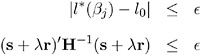
where l *( ² j ), s , and H are the log likelihood, the gradient, and the Hessian evaluated at the current parameter vector and » is a constant computed by the procedure. The first condition for convergence means that the log-likelihood function must be within ˆˆ of the correct value, and the second condition means that the gradient vector must be proportional to the restriction vector r .
When you request the LRCI option in the MODEL statement, PROC GENMOD computes profile likelihood confidence intervals for all parameters in the model, including the scale parameter, if there is one. The interval endpoints are displayed in a table as well as the values of the remaining parameters at the solution.
Wald Confidence Intervals
You can request that PROC GENMOD produce Wald confidence intervals for the parameters. The (1- ± )100% Wald confidence interval for a parameter ² is defined as
where z p is the 100 p th percentile of the standard normal distribution, ![]() is the parameter estimate, and
is the parameter estimate, and ![]() is the estimate of its standard error.
is the estimate of its standard error.
F Statistics
Suppose that D is the deviance resulting from fitting a generalized linear model and that D 1 is the deviance from fitting a submodel . Then, under appropriate regularity conditions, the asymptotic distribution of ( D 1 ˆ’ D ) / ![]() is chi-square with r degrees of freedom, where r is the difference in the number of parameters between the two models and
is chi-square with r degrees of freedom, where r is the difference in the number of parameters between the two models and ![]() is the dispersion parameter. If
is the dispersion parameter. If ![]() is unknown, and
is unknown, and ![]() is an estimate of
is an estimate of ![]() based on the deviance or Pearsons chi-square divided by degrees of freedom, then, under regularity conditions, ( n ˆ’ p )
based on the deviance or Pearsons chi-square divided by degrees of freedom, then, under regularity conditions, ( n ˆ’ p ) ![]() /
/ ![]() has an asymptotic chi-square distribution with n ˆ’ p degrees of freedom. Here, n is the number of observations and p is the number of parameters in the model that is used to estimate
has an asymptotic chi-square distribution with n ˆ’ p degrees of freedom. Here, n is the number of observations and p is the number of parameters in the model that is used to estimate ![]() . Thus, the asymptotic distribution of
. Thus, the asymptotic distribution of
is the F distribution with r and n ˆ’ p degrees of freedom, assuming that ( D 1 ˆ’ D ) / ![]() and ( n ˆ’ p )
and ( n ˆ’ p ) ![]() /
/ ![]() are approximately independent.
are approximately independent.
This F statistic is computed for the Type 1 analysis, Type 3 analysis, and hypothesis tests specified in CONTRAST statements when the dispersion parameter is estimated by either the deviance or Pearsons chi-square divided by degrees of freedom, as specified by the DSCALE or PSCALE option in the MODEL statement. In the case of a Type 1 analysis, model 0 is the higher-order model obtained by including one additional effect in model 1. For a Type 3 analysis and hypothesis tests, model 0 is the full specified model and model 1 is the sub-model obtained from constraining the Type III contrast or the user -specified contrast to be 0.
Lagrange Multiplier Statistics
When you select the NOINT or NOSCALE option, restrictions are placed on the intercept or scale parameters. Lagrange multiplier, or score, statistics are computed in these cases. These statistics assess the validity of the restrictions, and they are computed as
where s is the component of the score vector evaluated at the restricted maximum corresponding to the restricted parameter and ![]() . The matrix I is the information matrix, 1 refers to the restricted parameter, and 2 refers to the rest of the parameters.
. The matrix I is the information matrix, 1 refers to the restricted parameter, and 2 refers to the rest of the parameters.
Under regularity conditions, this statistic has an asymptotic chi-square distribution with one degree of freedom, and p -values are computed based on this limiting distribution.
If you set k =0 in a negative binomial model, s is the score statistic of Cameron and Trivedi (1998) for testing for overdispersion in a Poisson model against alternatives of the form V ( ¼ )= ¼ + k ¼ 2 .
Refer to Rao (1973, p. 417) for more details.
Predicted Values of the Mean
Predicted Values
A predicted value, or fitted value, of the mean ¼ i corresponding to the vector of covariates x i is given by
where g is the link function, regardless of whether x i corresponds to an observation or not. That is, the response variable can be missing and the predicted value is still computed for valid x i . In the case where x i does not correspond to a valid observation, x i is not checked for estimability. You should check the estimability of x i in this case in order to ensure the uniqueness of the predicted value of the mean. If there is an offset, it is included in the predicted value computation.
Confidence Intervals on Predicted Values
Approximate confidence intervals for predicted values of the mean can be computed as follows. The variance of the linear predictor ![]() is estimated by
is estimated by
where is the estimated covariance of ![]() .
.
Approximate 100(1 ˆ’ ± )% confidence intervals are computed as
where z p is the 100 p percentile of the standard normal distribution and g is the link function. If either endpoint in the argument is outside the valid range of arguments for the inverse link function, the corresponding confidence interval endpoint is set to missing.
Residuals
The GENMOD procedure computes three kinds of residuals. The raw residual is defined as
where y i is the i th response and ¼ i is the corresponding predicted mean.
The Pearson residual is the square root of the i th contribution to the Pearsons chi-square.
Finally, the deviance residual is defined as the square root of the contribution of the i th observation to the deviance, with the sign of the raw residual.
The adjusted Pearson, deviance, and likelihood residuals are defined by Agresti (1990), Williams (1987), and Davison and Snell (1991). These residuals are useful for outlier detection and for assessing the influence of single observations on the fitted model.
For the generalized linear model, the variance of the i th individual observation is given by
where ![]() is the dispersion parameter, w i is a user-specified prior weight (if not specified, w i = 1), ¼ i is the mean, and V ( ¼ i ) is the variance function. Let
is the dispersion parameter, w i is a user-specified prior weight (if not specified, w i = 1), ¼ i is the mean, and V ( ¼ i ) is the variance function. Let
for the i th observation, where g ² ( ¼ i ) is the derivative of the link function, evaluated at ¼ Let W e be the diagonal matrix with w i denoting the i th diagonal element. The weight matrix W e is used in computing the expected information matrix.
Define h i as the i th diagonal element of the matrix
The Pearson residuals, standardized to have unit asymptotic variance, are given by
The deviance residuals, standardized to have unit asymptotic variance, are given by
where d i is the square root of the contribution to the total deviance from observation i , and sign( y i ˆ’ ¼ i ) is 1 if y i ˆ’ ¼ i is positive and -1 if y i ˆ’ ¼ i is negative. The likelihood residuals are defined by
Multinomial Models
This type of model applies to cases where an observation can fall into one of k categories. Binary data occurs in the special case where k = 2. If there are m i observations in a subpopulation i , then the probability distribution of the number falling into the k categories y i = ( y i 1 ,y i 2 , y ik ) can be modeled by the multinomial distribution, defined in the Response Probability Distributions section (page 1650), with ˆ‘ j y ij = m i . The multinomial model is an ordinal model if the categories have a natural order.
The GENMOD procedure orders the response categories for ordinal multinomial models from lowest to highest by default. This is different from the binomial distribution, where the response probability for the lowest of the two categories is modeled. You can change the way GENMOD orders the response levels with the RORDER= option in the PROC GENMOD statement. The order that GENMOD uses is shown in the Response Profiles output table described in the section Response Profile on page 1685.
The GENMOD procedure supports only the ordinal multinomial model. If ( p i 1 , p i 2 , p ik ) are the category probabilities, the cumulative category probabilities are modeled with the same link functions used for binomial data. Let ![]() , r = 1, 2, , k ˆ’ 1 be the cumulative category probabilities (note that P ik = 1). The ordinal model is
, r = 1, 2, , k ˆ’ 1 be the cumulative category probabilities (note that P ik = 1). The ordinal model is
where ¼ 1 , ¼ 2 , ¼ k ˆ’ 1 are intercept terms that depend only on the categories and x i is a vector of covariates that does not include an intercept term. The logit, probit, and complementary log-log link functions g are available. These are obtained by specifying the MODEL statement options DIST=MULTINOMIAL and LINK=CUMLOGIT (cumulative logit), LINK=CUMPROBIT (cumulative probit), or LINK=CUMCLL (cumulative complementary log-log). Alternatively,
where F = g ˆ’ 1 is a cumulative distribution function for the logistic, normal, or extreme value distribution.
PROC GENMOD estimates the intercept parameters ¼ 1 , ¼ 2 , ¼ k ˆ’ 1 and regression parameters ² by maximum likelihood.
The subpopulations i are defined by constant values of the AGGREGATE= variable. This has no effect on the parameter estimates, but it does affect the deviance and Pearson chi-square statistics; it also affects parameter estimate standard errors if you specify the SCALE=DEVIANCE or SCALE=PEARSON options.
Generalized Estimating Equations
Let y ij , j = 1, , n i , i = 1, , K represent the j th measurement on the i th subject. There are n i measurements on subject i and ![]() total measurements.
total measurements.
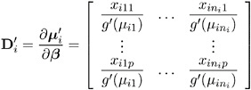
Correlated data are modeled using the same link function and linear predictor setup (systematic component) as the independence case. The random component is described by the same variance functions as in the independence case, but the covariance structure of the correlated measurements must also be modeled. Let the vector of measurements on the i th subject be Y i = [ y i 1 , , y in i ] ² with corresponding vector of means µ i = [ µ i 1 , , µ ini ] ² and let V i be the covariance matrix of Y i . Let the vector of independent, or explanatory, variables for the j th measurement on the i th subject be
The Generalized Estimating Equation of Liang and Zeger (1986) for estimating the p 1 vector of regression parameters ² is an extension of the independence estimating equation to correlated data and is given by
where
Since
where g is the link function, the p n i matrix of partial derivatives of the mean with respect to the regression parameters for the i th subject is given by
Working Correlation Matrix
Let R i ( ± ) be an n i n i working correlation matrix that is fully specified by the vector of parameters ± . The covariance matrix of Y i is modeled as
where A i is an n i n i diagonal matrix with v ( ¼ ij ) as the j th diagonal element and W i is an n i n i diagonal matrix with w ij as the j th diagonal where w ij is a weight specified with the WEIGHT statement. If there is no WEIGHT statement, w ij = 1 for all i and j . If R i ( ± ) is the true correlation matrix of Y i , then V i is the true covariance matrix of Y i .
The working correlation matrix is usually unknown and must be estimated. It is estimated in the iterative fitting process using the current value of the parameter vector ² to compute appropriate functions of the Pearson residual
If you specify the working correlation as R = I , which is the identity matrix, the GEE reduces to the independence estimating equation.
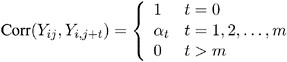
Following are the structures of the working correlation supported by the GENMOD procedure and the estimators used to estimate the working correlations .
| Working Correlation Structure | Estimator | |
|---|---|---|
| Fixed | ||
| Corr( Y ij ,Y ik ) = r jk where r jk is the jk th element of a constant, user-specified correlation matrix R . | The working correlation is not estimated in this case. | |
| Independent | ||
| | The working correlation is not estimated in this case. | |
| m -dependent | ||
| | | |
| Exchangeable | ||
| | | |
| Unstructured | ||
| | | |
| Autoregressive AR(1) | ||
| | | |
Dispersion Parameter
The dispersion parameter ![]() is estimated by
is estimated by
where ![]() is the total number of measurements and p is the number of regression parameters.
is the total number of measurements and p is the number of regression parameters.
The square root of ![]() is reported by PROC GENMOD as the scale parameter in the Analysis of GEE Parameter Estimates Model-Based Standard Error Estimates output table.
is reported by PROC GENMOD as the scale parameter in the Analysis of GEE Parameter Estimates Model-Based Standard Error Estimates output table.
Fitting Algorithm
The following is an algorithm for fitting the specified model using GEEs. Note that this is not in general a likelihood-based method of estimation, so that inferences based on likelihoods are not possible for GEE methods .
-
Compute an initial estimate of ² with an ordinary generalized linear model assuming independence.
-
Compute the working correlations R based on the standardized residuals, the current ² , and the assumed structure of R .
-
Compute an estimate of the covariance:
-
Update ² :
-
Iterate steps 2-4 until convergence
Missing Data
Refer to Diggle, Liang, and Zeger (1994, Chapter 11) for a discussion of missing values in longitudinal data. Suppose that you intend to take measurements Y i 1 , , Y in for the i th unit. Missing values for which Y ij are missing whenever Y ik is missing for all j k are called dropouts . Otherwise, missing values that occur intermixed with nonmissing values are intermittent missing values. The GENMOD procedure can estimate the working correlation from data containing both types of missing values using the all available pairs method, in which all nonmissing pairs of data are used in the moment estimators of the working correlation parameters defined previously.
For example, for the unstructured working correlation model,
where the sum is over the units that have nonmissing measurements at times j and k , and K ² is the number of units with nonmissing measurements at j and k . Estimates of the parameters for other working correlation types are computed in a similar manner, using available nonmissing pairs in the appropriate moment estimators.
The contribution of the i th unit to the parameter update equation is computed by omitting the elements of ( Y i ˆ’ ¼ i ), the columns of ![]() , and the rows and columns of V i corresponding to missing measurements.
, and the rows and columns of V i corresponding to missing measurements.
Parameter Estimate Covariances
The model-based estimator of Cov( ![]() ) is given by
) is given by
where
This is the GEE equivalent of the inverse of the Fisher information matrix that is often used in generalized linear models as an estimator of the covariance estimate of the maximum likelihood estimator of ² . It is a consistent estimator of the covariance matrix of ![]() if the mean model and the working correlation matrix are correctly specified.
if the mean model and the working correlation matrix are correctly specified.
The estimator
is called the empirical , or robust , estimator of the covariance matrix of ![]() where
where
It has the property of being a consistent estimator of the covariance matrix of ![]() , even if the working correlation matrix is misspecified, that is, if Cov( Y i ) V i . In computing M , ² and
, even if the working correlation matrix is misspecified, that is, if Cov( Y i ) V i . In computing M , ² and ![]() are replaced by estimates, and Cov( Y i ) is replaced by the estimate
are replaced by estimates, and Cov( Y i ) is replaced by the estimate
Multinomial GEEs
Lipsitz, Kim, and Zhao (1994) and Miller, Davis, and Landis (1993) describe how to extend GEEs to multinomial data. Currently, only the independent working correlation is available for multinomial models in PROC GENMOD.
Alternating Logistic Regressions
If the responses are binary (that is, they take only two values), then there is an alternative method to account for the association among the measurements. The Alternating Logistic Regressions (ALR) algorithm of Carey, Zeger, and Diggle (1993) models the association between pairs of responses with log odds ratios, instead of with correlations, as ordinary GEEs do.
For binary data, the correlation between the j th and k th response is, by definition,
The joint probability in the numerator satisfies the following bounds, by elementary properties of probability, since ¼ ij = Pr( Y ij = 1):
The correlation, therefore, is constrained to be within limits that depend in a complicated way on the means of the data.
The odds ratio, defined as
is not constrained by the means and is preferred, in some cases, to correlations for binary data.
The ALR algorithm seeks to model the logarithm of the odds ratio, ³ ijk = log( OR ( Y ij ,Y ik )), as
where ± is a q 1 vector of regression parameters and z ijk is a fixed, specified vector of coefficients.
The parameter ³ ijk can take any value in ( ˆ’ˆ , ˆ ) with ³ ijk = 0 corresponding to no association.
The log odds ratio, when modeled in this way with a regression model, can take different values in subgroups defined by z ijk . For example, z ijk can define subgroups within clusters, or it can define ˜block effects between clusters.
You specify a GEE model for binary data using log odds ratios by specifying a model for the mean, as in ordinary GEEs, and a model for the log odds ratios. You can use any of the link functions appropriate for binary data in the model for the mean, such as logistic, probit, or complementary log-log. The ALR algorithm alternates between a GEE step to update the model for the mean and a logistic regression step to update the log odds ratio model. Upon convergence, the ALR algorithm provides estimates of the regression parameters for the mean, ² , the regression parameters for the log odds ratios, ± , their standard errors, and their covariances.
Specifying Log Odds Ratio Models
Specifying a regression model for the log odds ratio requires you to specify rows of the z -matrix z ijk for each cluster i and each unique within-cluster pair ( j, k ). The GENMOD procedure provides several methods of specifying z ijk . These are controlled by the LOGOR= keyword and associated options in the REPEATED statement. The supported keywords and the resulting log odds ratio models are described as follows.
| EXCH | exchangeable log odds ratios. In this model, the log odds ratio is a constant for all clusters i and pairs ( j, k ). The parameter ± is the common log odds ratio. | |
| FULLCLUST | fully parameterized clusters. Each cluster is parameterized in the same way, and there is a parameter for each unique pair within clusters. If a complete cluster is of size n , then there are The elements of ± correspond to log odds ratios for cluster pairs in the following order: | |
| Pair | Parameter | |
| (1,2) | Alpha1 | |
| (1,3) | Alpha2 | |
| (1,4) | Alpha3 | |
| (2.3) | Alpha4 | |
| (2,4) | Alpha5 | |
| (3,4) | Alpha6 | |
| LOGORVAR( variable ) | log odds ratios by cluster. The argument variable is a variable name that defines the ˜block effects between clusters. The log odds ratios are constant within clusters, but they take a different value for each different value of the variable . For example, if Center is a variable in the input data set taking a different value for k treatment centers, then specifying LOGOR=LOGORVAR(Center) requests a model with different log odds ratios for each of the k centers, constant within center. | |
| NESTK | k -nested log odds ratios. You must also specify the SUBCLUST= variable option to define subclusters within clusters. Within each cluster, PROC GENMOD computes a log odds ratio parameter for pairs having the same value of variable for both members of the pair and one log odds ratio parameter for each unique combination of different values of variable . | |
| NEST1 | 1-nested log odds ratios. You must also specify the SUBCLUST= variable option to define subclusters within clusters. There are two log odds ratio parameters for this model. Pairs having the same value of variable correspond to one parameter; pairs having different values of variable correspond to the other parameter. For example, if clusters are hospitals and subclusters are wards within hospitals , then patients within the same ward have one log odds ratio parameter, and patients from different wards have the other parameter. | |
| ZFULL | specifies the full z -matrix. You must also specify a SAS data set containing the z -matrix with the ZDATA= data-set-name option. Each observation in the data set corresponds to one row of the z -matrix. You must specify the ZDATA data set as if all clusters are complete, that is, as if all clusters are the same size and there are no missing observations. The ZDATA data set has K [ n max ( n max ˆ’ 1) /2] observations, where K is the number of clusters and n max is the maximum cluster size. If the members of cluster i are ordered as 1, 2, ..., n , then the rows of the z -matrix must be specified for pairs in the order (1, 2), (1, 3), ..., (1, n ), (2, 3), ..., (2, n ), ..., ( n ˆ’ 1, n ). The variables specified in the REPEATED statement for the SUBJECT effect must also be present in the ZDATA= data set to identify clusters. You must specify variables in the data set that define the columns of the z -matrix by the ZROW= variable-list option. If there are q columns, ( q variables in variable-list ), then there are q log odds ratio parameters. You can optionally specify variables indicating the cluster pairs corresponding to each row of the z -matrix with the YPAIR=( variable1, variable2 ) option. If you specify this option, the data from the ZDATA data set is sorted within each cluster by variable1 and variable2 . See Example 31.6 for an example of specifying a full z -matrix. | |
| ZREP | replicated z -matrix. You specify z -matrix data exactly as you do for the ZFULL case, except that you specify only one complete cluster. The z -matrix for the one cluster is replicated for each cluster. The number of observations in the ZDATA data set is | |
| ZREP(matrix) | direct input of the replicated z -matrix. You specify the z -matrix for one cluster with the syntax LOGOR=ZREP (( y 1 y 2 ) z 1 z 2 ... z q , ...), where y 1 and y 2 are numbers representing a pair of observations and the values z 1 , z 2 , ..., z q make up the corresponding row of the z -matrix. The number of rows specified is LOGOR = ZREP((1 2) 1 0, (1 3) 1 0, (1 4) 1 0, (2 3) 1 1, (2 4) 1 1, (3 4) 1 1) specifies the | |
Generalized Score Statistics
Boos (1992) and Rotnitzky and Jewell (1990) describe score tests applicable to testing L ² = in GEEs, where L is a user-specified r p contrast matrix or a contrast for a Type 3 test of hypothesis.
Let ![]() be the regression parameters resulting from solving the GEE under the restricted model L ² = , and let S (
be the regression parameters resulting from solving the GEE under the restricted model L ² = , and let S ( ![]() ) be the generalized estimating equation values at
) be the generalized estimating equation values at ![]() .
.
The generalized score statistic is
where m is the model-based covariance estimate and e is the empirical covariance estimate. The p -values for T are computed based on the chi-square distribution with r degrees of freedom.
Assessment of Models Based on Aggregates of Residuals (Experimental)
Lin, Wei, and Ying (2002) present graphical and numerical methods for model assessment based on the cumulative sums of residuals over certain coordinates (e.g., covariates or linear predictors) or some related aggregates of residuals. The distributions of these stochastic processes under the assumed model can be approximated by the distributions of certain zero-mean Gaussian processes whose realizations can be generated by simulation. Each observed residual pattern can then be compared, both graphically and numerically, with a number of realizations from the null distribution. Such comparisons enable you to assess objectively whether the observed residual pattern reflects anything beyond random fluctuation. These procedures are useful in determining appropriate functional forms of covariates and link function. You use the ASSESSASSESSMENT statement to perform this kind of model-checking with cumulative sums of residuals, moving sums of residuals, or LOWESS smoothed residuals. See Example 31.8 and Example 31.9 for examples of model assessment.
Let the model for the mean be
where ¼ i is the mean of the response y i and x i is the vector of covariates for the i th observation. Denote the raw residual resulting from fitting the model as
and let x ij be the value of the j th covariate in the model for observation i . Then to check the functional form of the j th covariate, consider the cumulative sum of residuals with respect to x ij
where I () is the indicator function. For any x , W j ( x ) is the sum of the residuals with values of x j less than or equal to x .
Denote the score, or gradient vector by
where ½ ( r ) = g ˆ’ 1 ( r ), and
Let J be the Fisher information matrix
Define
where
and Z i are independent N (0, 1) random variables. Then the conditional distribution of j ( x ), given ( y i , x i ), i = 1, , n , under the null hypothesis H that the model for the mean is correct, is the same asymptotically as n ’ ˆ as the unconditional distribution of W j ( x ) (Lin, Wei, and Ying, 2002).
You can approximate realizations from the null hypothesis distribution of W j ( x ) by repeatedly generating normal samples Z i , i = 1, ... , n while holding ( y i , x i ), i = 1, , n at their observed values and computing j ( x ) for each sample.
You can assess the functional form of covariate j by plotting a few realizations of j ( x ) on the same plot as the observed W j ( x ) and visually comparing to see how typical the observed W j ( x ) is of the null distribution samples.
You can supplement the graphical inspection method with a Kolmogorov-type supremum test. Let s j be the observed value of S j = sup x W j ( x ). The p -value Pr[ S j s j ] is approximated by Pr[ j s j ], where j = sup x j ( x ) . Pr[ j s j ] is estimated by generating realizations of j ( . ) (1,000 is the default number of realizations).
You can check the link function instead of the j th covariate by using values of the linear predictor x i ² ![]() in place of values of the j th covariate x ij . The graphical and numerical methods described above are then sensitive to inadequacies in the link function.
in place of values of the j th covariate x ij . The graphical and numerical methods described above are then sensitive to inadequacies in the link function.
An alternative aggregate of residuals is the moving sum statistic
If you specify the keyword WINDOW( b ), then the moving sum statistic with window size b is used instead of the cumulative sum of residuals, with I ( x ˆ’ b x ij x ) replacing I ( x ij x ) above.
If you specify the keyword LOWESS( f ), LOWESS smoothed residuals are used in the formulas above, where f is the fraction of the data to be used at a given point. If f is not specified, f = 1/3 is used. Define, for data ( Y i , X i ), i = 1, , n , r as the nearest integer to nf and h as the r th smallest among X i ˆ’ x , i = 1, , n . Let
where
Define
where
Then the LOWESS estimate of Y at x is defined by
LOWESS smoothed residuals for checking the functional form of the j th covariate are defined by replacing Y i with e i and X i with x ij . To implement the graphical and numerical assessment methods, I ( x ij x ) is replaced with ![]() in the formulas for W j ( x ) and j ( x ).
in the formulas for W j ( x ) and j ( x ).
You can perform the model checking described above for marginal models for dependent responses fit by generalized estimating equations (GEEs). Let y ik denote the k th measurement on the i th cluster, i = 1, ..., K , k = 1, ..., n i , and x ik the corresponding vector of covariates. The marginal mean of the response ¼ ik = E( y ik ) is assumed to depend on the covariate vector by
where g is the link function.
Define the vector of residuals for the i th cluster as
You use the following extension of W j ( x ) defined above to check the functional form of the j th covariate:
where x ikj is the j th component of x ik .
The null distribution of W j ( x ) can be approximated by the conditional distribution of
where ![]() and
and ![]() are defined as in the section Generalized Estimating Equations on page 1672 with the unknown parameters replaced by their estimated values,
are defined as in the section Generalized Estimating Equations on page 1672 with the unknown parameters replaced by their estimated values,
and Z i , i = 1, , K , are independent N (0 , 1) random variables. You replace x ik j with the linear predictor x ² ik ![]() in the preceding formulas to check the link function.
in the preceding formulas to check the link function.
Displayed Output
The following output is produced by the GENMOD procedure. Note that some of the tables are optional and appear only in conjunction with the REPEATED statement and its options or with options in the MODEL statement. For details, see the section ODS Table Names on page 1693.
Model Information
PROC GENMOD displays the following model information:
-
data set name
-
response distribution
-
link function
-
response variable name
-
offset variable name
-
frequency variable name
-
scale weight variable name
-
number of observations used
-
number of events if events/trials format is used for response
-
number of trials if events/trials format is used for response
-
sum of frequency weights
-
number of missing values in data set
-
number of invalid observations (for example, negative or 0 response values with gamma distribution or number of observations with events greater than trials with binomial distribution)
Class Level Information
If you use classification variables in the model, PROC GENMOD displays the levels of classification variables specified in the CLASS statement and in the MODEL statement. The levels are displayed in the same sorted order used to generate columns in the design matrix.
Response Profile
If you specify an ordinal model for the multinomial distribution, a table titled Response Profile is displayed containing the ordered values of the response variable and the number of occurrences of the values used in the model.
Iteration History for Parameter Estimates
If you specify the ITPRINT model option, PROC GENMOD displays a table containing the following for each iteration in the Newton-Raphson procedure for model fitting:
-
iteration number
-
ridge value
-
log likelihood
-
values of all parameters in the model
Criteria for Assessing Goodness of Fit
PROC GENMOD displays the following criteria for assessing goodness of fit:
-
degrees of freedom for deviance and Pearsons chi-square, equal to the number of observations minus the number of regression parameters estimated
-
deviance
-
deviance divided by degrees of freedom
-
scaled deviance
-
scaled deviance divided by degrees of freedom
-
Pearsons chi-square
-
Pearsons chi-square divided by degrees of freedom
-
scaled Pearsons chi-square
-
scaled Pearsons chi-square divided by degrees of freedom
-
log likelihood
Last Evaluation of the Gradient
If you specify the model option ITPRINT, the GENMOD procedure displays the last evaluation of the gradient vector.
Last Evaluation of the Hessian
If you specify the model option ITPRINT, the GENMOD procedure displays the last evaluation of the Hessian matrix.
Analysis of (Initial) Parameter Estimates
The Analysis of (Initial) Parameter Estimates table contains the results from fitting a generalized linear model to the data. If you specify the REPEATED statement, these GLM parameter estimates are used as initial values for the GEE solution. For each parameter in the model, PROC GENMOD displays the following:
-
the parameter name
-
the variable name for continuous regression variables
-
the variable name and level for classification variables and interactions involving classification variables
-
SCALE for the scale variable related to the dispersion parameter
-
-
degrees of freedom for the parameter
-
estimate value
-
standard error
-
Wald chi-square value
-
p -value based on the chi-square distribution
-
confidence limits (Wald or profile likelihood) for parameters
Estimated Covariance Matrix
If you specify the model option COVB, the GENMOD procedure displays the estimated covariance matrix, defined as the inverse of the information matrix at the final iteration. This is based on the expected information matrix if the EXPECTED option is specified in the MODEL statement. Otherwise, it is based on the Hessian matrix used at the final iteration. This is, by default, the observed Hessian unless altered by the SCORING option in the MODEL statement.
Estimated Correlation Matrix
If you specify the CORRB model option, PROC GENMOD displays the estimated correlation matrix. This is based on the expected information matrix if the EXPECTED option is specified in the MODEL statement. Otherwise, it is based on the Hessian matrix used at the final iteration. This is, by default, the observed Hessian unless altered by the SCORING option in the MODEL statement.
Iteration History for LR Confidence Intervals
If you specify the ITPRINT and LRCI model options, PROC GENMOD displays an iteration history table for profile likelihood-based confidence intervals. For each parameter in the model, PROC GENMOD displays the following:
-
parameter identification number
-
iteration number
-
log likelihood value
-
parameter values
Likelihood Ratio-Based Confidence Intervals for Parameters
If you specify the LRCI and the ITPRINT options in the MODEL statement, a table is displayed summarizing profile likelihood-based confidence intervals for all parameters. The table contains the following for each parameter in the model:
-
confidence coefficient
-
parameter identification number
-
lower and upper endpoints of confidence intervals for the parameter
-
values of all other parameters at the solution
LR Statistics for Type 1 Analysis
If you specify the TYPE1 model option, a table containing the following is displayed for each effect in the model:
-
name of effect
-
deviance for the model including the effect and all previous effects
-
degrees of freedom for the effect
-
likelihood ratio statistic for testing the significance of the effect
-
p -value computed from the chi-square distribution with effect degrees of freedom
If you specify either the SCALE=DEVIANCE or SCALE=PEARSON option in the MODEL statement, columns containing the following are displayed:
-
name of effect
-
deviance for the model including the effect and all previous effects
-
numerator degrees of freedom
-
denominator degrees of freedom
-
chi-square statistic for testing the significance of the effect
-
p -value computed from the chi-square distribution with numerator degrees of freedom
-
F statistic for testing the significance of the effect
-
p -value based on the F distribution
Iteration History for Type 3 Contrasts
If you specify the model options ITPRINT and TYPE3, an iteration history table is displayed for fitting the model with Type 3 contrast constraints for each effect. The table contains the following:
-
effect name
-
iteration number
-
ridge value
-
log likelihood
-
values of all parameters
LR Statistics for Type 3 Analysis
If you specify the TYPE3 model option, a table containing the following is displayed for each effect in the model:
-
name of the effect
-
likelihood ratio statistic for testing the significance of the effect
-
degrees of freedom for effect
-
p -value computed from the chi-square distribution
If you specify either the SCALE=DEVIANCE or SCALE=PEARSON option in the MODEL statement, columns containing the following are displayed:
-
name of the effect
-
likelihood ratio statistic for testing the significance of the effect
-
F statistic for testing the significance of the effect
-
numerator degrees of freedom
-
denominator degrees of freedom
-
p -value based on the F distribution
-
p -value computed from the chi-square distribution with numerator degrees of freedom
Wald Statistics for Type 3 Analysis
If you specify the TYPE3 and WALD model options, a table containing the following is displayed for each effect in the model:
-
name of effect
-
degrees of freedom for effect
-
Wald statistic for testing the significance of the effect
-
p -value computed from the chi-square distribution
Parameter Information
If you specify the ITPRINT, COVB, CORRB, WALDCI, or LRCI option in the MODEL statement, or if you specify a CONTRAST statement, a table is displayed that identifies parameters with numbers, rather than names, for use in tables and matrices where a compact identifier for parameters is helpful. For each parameter, the table contains the following:
-
a number that identifies the parameter
-
the parameter name, including level information for effects containing classification variables
Observation Statistics
If you specify the OBSTATS option in the MODEL statement, PROC GENMOD displays a table containing miscellaneous statistics. For each observation in the input data set, the following are displayed:
-
the value of the response variable, denoted by the variable name
-
the predicted value of the mean, denoted by PRED
-
the value of the linear predictor, denoted by XBETA. The value of an OFFSET variable is added to the linear predictor.
-
the estimated standard error of the linear predictor, denoted by STD
-
the value of the negative of the weight in the Hessian matrix at the final iteration, denoted by HESSWGT. This is the expected weight if the EXPECTED option is specified in the MODEL statement. Otherwise, it is the weight used in the final iteration. That is, it is the observed weight unless the SCORING= option has been specified.
-
approximate lower and upper endpoints for a confidence interval for the predicted value of the mean, denoted by LOWER and UPPER
-
raw residual, denoted by RESRAW
-
Pearson residual, denoted by RESCHI
-
deviance residual, denoted by RESDEV
-
standardized Pearson residual, denoted by STDRESCHI
-
standardized deviance residual, denoted by STDRESDEV
-
likelihood residual, denoted by RESLIK
ESTIMATE Statement Results
If you specify a REPEATED statement, the ESTIMATE statement results apply to the specified GEE model. Otherwise, they apply to the specified generalized linear model.
The following are displayed for each ESTIMATE statement:
-
contrast label
-
estimated value of the contrast
-
standard error of the estimate
-
significance level ±
-
(1 ˆ’ ± ) 100% confidence intervals for contrast
-
Wald chi-square statistic for the contrast
-
p -value computed from the chi-square distribution
If you specify the EXP option, an additional row is displayed with statistics for the exponentiated value of the contrast.
CONTRAST Coefficients
If you specify the CONTRAST or ESTIMATE statement and you specify the E option, a table titled Coefficients For Contrast label is displayed, where label is the label specified in the CONTRAST statement. The table contains the following:
-
the contrast label
-
the rows of the contrast matrix
Iteration History for Contrasts
If you specify the ITPRINT option, an iteration history table is displayed for fitting the model with contrast constraints for each effect. The table contains the following for each contrast defined in a CONTRAST statement:
-
contrast label
-
iteration number
-
ridge value
-
log likelihood
-
values of all parameters
CONTRAST Statement Results
If you specify a REPEATED statement, the CONTRAST statement results apply to the specified GEE model. Otherwise, they apply to the specified generalized linear model.
The following are displayed for each CONTRAST statement:
-
contrast label
-
degrees of freedom for the contrast
-
likelihood ratio, score, or Wald statistic for testing the significance of the contrast. Score statistics are used in GEE models, likelihood ratio statistics are used in generalized linear models, and Wald statistics are used in both.
-
p -value computed from the chi-square distribution
-
the type of statistic computed for this contrast: Wald, LR, or score
If you specify either the SCALE=DEVIANCE or SCALE=PEARSON option for generalized linear models, columns containing the following are displayed:
-
contrast label
-
likelihood ratio statistic for testing the significance of the contrast
-
F statistic for testing the significance of the contrast
-
numerator degrees of freedom
-
denominator degrees of freedom
-
p -value based on the F distribution
-
p -value computed from the chi-square distribution with numerator degrees of freedom
LSMEANS Coefficients
If you specify the LSMEANS statement and you specify the E option, a table titled Coefficients for effect Least Squares Means is displayed, where effect is the effect specified in the LSMEANS statement. The table contains the following:
-
the effect names
-
the rows of least squares means coefficients
Least Squares Means
If you specify the LSMEANS statement a table titled Least Squares Means is displayed. The table contains the following:
-
the effect names
-
for each level of each effect,
-
the least squares mean estimate
-
standard error
-
chi-square value
-
p -value computed from the chi-square distribution
-
If you specify the DIFF option, a table titled Differences of Least Squares Means is displayed containing corresponding statistics for the differences between the least squares means for the levels of each effect.
GEE Model Information
If you specify the REPEATED statement, the following are displayed:
-
correlation structure of the working correlation matrix or the log odds ratio structure
-
within-subject effect
-
subject effect
-
number of clusters
-
correlation matrix dimension
-
minimum and maximum cluster size
Log Odds Ratio Parameter Information
If you specify the REPEATED statement and specify a log odds ratio model for binary data with the LOGOR= option, then a table is displayed showing the correspondence between data pairs and log odds ratio model parameters.
Iteration History for GEE Parameter Estimates
If you specify the REPEATED statement and the MODEL statement option ITPRINT, an iteration history table for GEE parameter estimates is displayed. The table contains the following:
-
parameter identification number
-
iteration number
-
values of all parameters
Last Evaluation of the Generalized Gradient and Hessian
If you specify the REPEATED statement and select ITPRINT as a model option, PROC GENMOD displays the last generalized gradient and Hessian matrix in the GEE iterative parameter estimation process.
GEE Parameter Estimate Covariance Matrices
If you specify the REPEATED statement and the COVB option, PROC GENMOD displays both model-based and empirical parameter estimate covariance matrices.
GEE Parameter Estimate Correlation Matrices
If you specify the REPEATED statement and the CORRB option, PROC GENMOD displays both model-based and empirical parameter estimate covariance matrices.
GEE Working Correlation Matrix
If you specify the REPEATED statement and the CORRW option, PROC GENMOD displays the exchangeable working correlation matrix.
Analysis of GEE Parameter Estimates
If you specify the REPEATED statement, PROC GENMOD uses empirical standard error estimates to compute and display the following for each parameter in the model:
-
the parameter name
-
the variable name for continuous regression variables
-
the variable name and level for classification variables and interactions involving classification variables
-
Scale for the scale variable related to the dispersion parameter
-
-
parameter estimate
-
standard error
-
95% confidence interval
-
Z score and p -value
If you specify the MODELSE option in the REPEATED statement, a table based on model-based standard errors is also produced.
GEE Observation Statistics
If you specify the OBSTATS option in the REPEATED statement, PROC GENMOD displays a table containing miscellaneous statistics. For each observation in the input data set, the following are displayed:
-
the value of the response variable and all other variables in the model, denoted by the variable names
-
the predicted value of the mean, denoted by PRED
-
the value of the linear predictor, denoted by XBETA
-
the standard error of the linear predictor, denoted by STD
-
confidence limits for the predicted values, denoted by LOWER and UPPER
-
raw residual, denoted by RESRAW
-
Pearson residual, denoted by RESCHI
ODS Table Names
PROC GENMOD assigns a name to each table that it creates. You can use these names to reference the table when using the Output Delivery System (ODS) to select tables and create output data sets. These names are listed in the following table. For more information on ODS, see Chapter 14, Using the Output Delivery System.
| ODS Table Name | Description | Statement | Option |
|---|---|---|---|
| AssessmentSummary (experimental) | Model assessment summary | ASSESS | default |
| ClassLevels | Class variable levels | CLASS | default |
| Contrasts | Tests of contrasts | CONTRAST | default |
| ContrastCoef | Contrast coefficients | CONTRAST | E |
| ConvergenceStatus | Convergence status | MODEL | default |
| CorrB | Parameter estimate correlation matrix | MODEL | CORRB |
| CovB | Parameter estimate covariance matrix | MODEL | COVB |
| Estimates | Estimates of contrasts | ESTIMATE | default |
| EstimateCoef | Contrast coefficients | ESTIMATE | E |
| GEEEmpPEst | GEE parameter estimates with empirical standard errors | REPEATED | default |
| GEELogORInfo | GEE log odds ratio model information | REPEATED | LOGOR= |
| GEEModInfo | GEE model information | REPEATED | default |
| GEEModPEst | GEE parameter estimates with model-based standard errors | REPEATED | MODELSE |
| GEENCorr | GEE model-based correlation matrix | REPEATED | MCORRB |
| GEENCov | GEE model-based covariance matrix | REPEATED | MCOVB |
| GEERCorr | GEE empirical correlation matrix | REPEATED | ECORRB |
| GEERCov | GEE empirical covariance matrix | REPEATED | ECOVB |
| GEEWCorr | GEE working correlation matrix | REPEATED | CORRW |
| IterContrasts | Iteration history for contrasts | MODEL CONTRAST | ITPRINT |
| IterLRCI | Iteration history for likelihood ratio confidence intervals | MODEL | LRCI ITPRINT |
| IterParms | Iteration history for parameter estimates | MODEL | ITPRINT |
| IterParmsGEE | Iteration history for GEE parameter estimates | MODEL REPEATED | ITPRINT |
| IterType3 | Iteration history for Type 3 statistics | MODEL | TYPE3 ITPRINT |
| LRCI | Likelihood ratio confidence intervals | MODEL | LRCI ITPRINT |
| LSMeanCoef | Coefficients for least squares means | LSMEANS | E |
| LSMeanDiffs | Least squares means differences | LSMEANS | DIFF |
| LSMeans | Least squares means | LSMEANS | default |
| LagrangeStatistics | Lagrange statistics | MODEL | NOINT NOSCALE |
| LastGEEGrad | Last evaluation of the generalized gradient and Hessian | MODEL REPEATED | ITPRINT |
| LastGradHess | Last evaluation of the gradient and Hessian | MODEL | ITPRINT |
| LinDep | Linearly dependent rows of contrasts | CONTRAST [*] | default |
| ModelInfo | Model information | MODEL | default |
| Modelfit | Goodness-of-fit statistics | MODEL | default |
| NObs | Number of observations summary | default | |
| NonEst | Nonestimable rows of contrasts | CONTRAST [*] | default |
| ObStats | Observation-wise statistics | MODEL | OBSTATS CL PREDICTED RESIDUALS XVARS |
| ParameterEstimates | Parameter estimates | MODEL | default |
| ParmInfo | Parameter indices | MODEL [*] | default |
| ResponseProfiles | Frequency counts for multinomial models | MODEL | DIST=MULTINOMIAL |
| Type1 | Type 1 tests | MODEL | TYPE1 |
| Type3 | Type 3 tests | MODEL | TYPE3 |
| [*] Depends on data. | |||
ODS Graphics (Experimental)
This section describes the use of ODS for creating statistical graphs with the GENMOD procedure. These graphics are experimental in this release, meaning that both the graphical results and the syntax for specifying them are subject to change in a future release.
To request these graphs you must specify the ODS GRAPHICS statement in addition to the ASSESS statement and options. For more information on the ASSESS statement, see the ASSESS Statement section on page 1627. For more information on the ODS GRAPHICS statement, see Chapter 15, Statistical Graphics Using ODS.
ODS Graph Names
PROC GENMOD assigns a name to each graph it creates using ODS. You can use these names to reference the graphs when using ODS. The names are listed in Table 31.4 .
To request these graphs, you must specify the ODS GRAPHICS statement in addition to the options indicated in Table 31.4.
| ODS Graph Name | Description | Statement | Option |
|---|---|---|---|
| CumResidPanel | Panel plot of aggregates of residuals | ASSESS | CRPANEL |
| CumulativeResiduals | Model assessment based on aggregates of residuals | ASSESS | default |
EAN: N/A
Pages: 105